YouTube channel, College Humor, has a game show series called 'Um, Actually' - a game of nerdy corrections, and general nerd trivia.
One of the 'shiny questions' involves putting things is order, for example, putting space ships or fictional creatures in order by size.
The way the scoring works (as far as I can tell) is you get one point for each item you put in the right 'position'. So if you guess (1,3,2,4), then you would get 2 points for getting 1 and 4 in the correct position.
The problem was, in the creatures game, there was this one creature which looked like a single-celled organism, but was actually the size of a galaxy (or something), making it the largest.
So suppose you get everything else in the right order, but you fell for the trap and put this surprisingly massive organism as smallest e.g. (2,3,4,1)
In that case, everything is in the wrong position, so no points. But I would argue since all but one are in the right order you should only lose one point.
The FineBros channel does a similar game - e.g. put the top 10 most liked videos of 2019 in order. Under their scoring system, you get 2 points if an entry is in the right position, and 1 point if it's off by one. So (1,3,2,4) would be worth 6 points and (2,3,4,1) would be worth 3 points
This is slightly better, but you still have a case where you can lose significant points for getting just one or two entries out of place. For example, if you had (3,4,5,6,7,1,2), then you would get 0 points, even tho 5 of 7 are in the right order.
So, can we come up with a better scoring system?
Levenshtein Distance
The first things that comes to mind is Levenshtein or 'minimum edit' distance.
This measures the distance between two strings (words) based on the minimum number of edits to get from one to the other. In this context, an edit is a single character addition (cats -> chats), deletion (cats -> cat), or substitution (cats -> bats)
Now, this doesn't seem quite relevant to our problem; we're not adding, deleting, or substituting, we're swapping. For Levenshtein, a swap would be considered a deletion + an addition (or 2 substitutions) e.g. cats -> cas -> cast
We could calculate the Levenshtein distance and just divide it by 2 - effectively treat delete+add (2 edits) as equivalent to a swap (1 edit). Or else, we can just take the general principle of finding the minimum number of swaps required to get from the guess solution to the correct order.
As for the actual score, we can take the number of entries in the list (N) minus the minimum number of swaps.
So for our original examples, (1,3,2,4) is worth 3, and (2,3,4,1) is also worth 3.
In the latter case, 1 wasn't 'swapped' with an actual element, but you could think of it as a swap with an implied 'null' element - (..,null,1,2,3,4,null,..) -> (..,null,null,2,3,4,1,null,...)
Dynamic Programming
Dynamic programming is an approach to solving a certain class of problem which would take a ridiculous amount of time to solve by brute force. With dynamic programming, these problems can be solved in a more reasonable amount of time by breaking them down and solving recursively.
One of the classic problem in dynamic programming is - find the longest increasing sub-sequence in a list of numbers?
For example, in (2,3,1,7,4,9,5,8) the longest increasing sub-sequence would be (2,3,4,5,8). So in this case, we might say the score is 5/8
Going back to our other examples, (1,3,2,4) would have sub-sequence (1,2,4) or (1,3,4), worth 3 in either case. And (2,3,4,1) would be (2,3,4) which is also worth 3
Weighted Error
This is all well and good, but doesn't it feel like (2,3,4,1) is 'more wrong' than (1,3,2,4). Each has one element out of order, but in the former that one element if further from where it's 'supposed' to be.
One correction might be to calculate the error as sum[abs(x-x')] where x is the position of an element, and x' is where it's supposed to be. So (1,3,2,4) would be (abs(1-1) + abs(3-2) + abs(2-3) + abs(4-4)) = 2
However, this is flawed. For the (2,3,4,1) example, the error comes out at 6. Once again, we're being penalised for all the elements that are in the right order but off-by-one
So a slight modification would be to only calculate the error for those elements which are out of place - that is, find the longest sub-sequence, and then calculate the error for all elements which don't belong to that sub-sequence.
For (1,3,2,4) the error would be 1 and for (2,3,4,1) it would be 3
But how do we get from the error to the actual score?
We can start by calculating the maximum error, then subtracting the calculated error from it. So what's the maximum error?
The most wrong you can be would be to get everything in the wrong order - i.e. all elements reversed. So if we have N elements, the error would be
abs(1 - N) + abs(2 - N-1) + ... + abs(N -1) = (N - 1) + (N - 3) + ... + (N - 1) = 4 * (N - 2)
Actually, there's a subtle flaw in this reasoning - even if all the elements are reversed, there is technically a longest sub-sequence of 1, so one of the entries shouldn't count towards the maximum error. The element we chose as the 1 correct one will affect the maximum error. If we chose the first element in the sequence, the max error is reduced by N-1, whereas if we chose one from the middle the max error is reduced by 1 or 0 (depending if there is an odd or even number of elements)
For simplicity, we'll just assume the middle entry and say max error adjustment is 0
So going back once more to our original examples, (1,3,2,4) has a score of 8 - 1 = 7, and (2,3,4,1) has a score of 8 - 3 = 5, making the latter 'more wrong' as desired.
Conclusion
I'm not sure if there was a point to all this. I don't think this is useful outside of scoring this particular kind of game.
It might be interesting to run an neural net or genetic algorithm or similar using this as the score function. I'd be interested to see how a neural net performed at sorting, in terms of performance and correctness.
But anyway,
Chris.

Showing posts with label algorithm. Show all posts
Showing posts with label algorithm. Show all posts
Monday, December 30, 2019

Sunday, July 31, 2016
Barber Queue
Time was when I needed a hair cut, I'd go at noon on a weekday, when the barber's is typically empty. One of the perks of being unemployed.
But these days I have to get my haircuts on Saturdays, before noon. Which is bad enough in itself - ideally I'd never see Saturday mornings at all. And to make matters worse, Saturday morning is also when the barbers is at its busiest.
Hence, I found myself sat in the waiter area of a barbershop for the best part of an hour. But this got me thinking about how queuing works at a barbers.
First In Who's Next?
At its core, the barber's queue is just a first-in first-out (FIFO) queue. But it has two interesting features:
1) The queue 'structure' is unordered
In general the queue 'structure' will be a waiting area with a bunch of seats. When someone new joins the queue, they're free to sit wherever. In fact, odds are, they'll pick a seat in a similar way to how men choose urinals - attempting to maximise personal space.
But the key point is, if someone were to just look at the queue, they wouldn't be able to tell who was next.
2) Each member of the queue knows whether or not they're next
Each member of the queue probably doesn't know who exactly is next, but they do know (with reasonable certainty) whether or not it's them.
The way this works is relatively simple - when you join the queue, you're aware of who was there when you arrived (and of anyone who arrives after you). So when all the people who were there ahead of you have gone, you know that you're next.
O(M G)
Okay, lets break out some Python (2.7)
Just for fun, let's say that the capacity of the queue is fixed - i.e. the waiting area has a fixed number of seats (though in practice, people are free to stand, as I was forced to).
Here, we're picking a 'seat' by iterate over the queue looking for the first empty slot (with a value of None). We could implement any seat picking strategy we fancy, this is just the easiest.
Once we find an empty seat, we create a new 'Member' object for the item, with position set to the current length of the queue, then increment the queue length. Also, if the queue has no empty slots, we raise an exception.
Of course, this isn't how things work in practice. The barber doesn't go to each person and say "are you next?", "how about you?". They simply say "who's next?", and the person who believes they are next steps forward. Though arguably, that's just equivalent to asking every member concurrently. But let's not complicate things.
So there we have it. Of course, this type of queue isn't really useful from a programming perspective.
All of insertion, deletion, and lookup are worst-case \(O(N)\), where N is the queue's capacity (not the number of people in the queue). Which is pretty much worse than all other types of queue.
Why do items keep disappearing from my queue?
Okay, let's move away from computer-sciencey queues. There are certain behaviours in real-world queues that don't apply or wouldn't make sense to programmatic queues.
For one, as I alluded to earlier, the capacity of the queue is not enforced - there's room for overflow, even if it means people have to stand.
But on the other hand, when a place does get that full, people are less likely to stick around.
In particular, we have two situations:
1) There's a non-zero probability that a person will not stick around if the queue is full or close to full. This probability will tend to be related to the length of the queue when that person arrives
\[p(not join) \sim f(capacity, length)\]
For example,
\[p(not join) = A\left(\frac{length}{capacity}\right) - C\]
where A and C are some constants relating to how likely the person is to stick around if the queue is 'full', and at what point they consider the place to be 'too full'.
2) There's a non-zero probability that a person already in the queue will leave before they're served. This probability will typically depend on how long the person has been waiting, and how many people are still ahead of them
\[p(leave) \sim g(wait, position)\]
It's interesting because as time passes, wait increases, but position decreases. So how the probability evolves depends on how those factors balance against one another.
In particular, the probability evolution will likely depend on how each particular person responds to the sunk-cost fallacy - i.e. are they the sort to think "well, I've waited this long, I might as well see it through to the end", or do they think "this is taking too long, I've got better things to do with my time"?
For the sake of arguing, lets go with an exponential function for the general form.
For a sunk-cost person we might have
\[p(leave) = B \cdot \exp\left(-d\cdot \frac{wait}{position}\right)\]
This is a function where p goes to zero as position goes to zero or wait goes to infinity (B and d are some arbitrary constants).

Whereas for a non-sunk-cost person we might have
\[p(leave) = B \cdot \exp\left(-\frac{d}{wait \cdot position}\right)\]
This is a function where p goes to zero as position goes to zero, but goes to one as wait goes to infinity.
This gives us an interesting graph

Because 'position' is discrete you get this nice step function, with intervals of the probability steadily rising, then suddenly dropping. We can also see that there's a point at which probability of leaving is maximum, around the time you're in the middle of the queue. Which seems plausible.
We also have situations where a person will leave and come back later. But since, when they come back, they have to join the back of the queue, they're mathematically indistinguishable from a someone arriving for the first time.
One other complicating situation is people in groups. For example, if there's a parent and child ahead of you in the queue, the child is getting their hair cut by one member of staff, the parent is waiting; another member of staff asks 'who's next?' - is it you or the parent?
Situations like these add uncertainty into a member's queue position, and by extension their knowledge of whether they're next.
In that situation, we might wait to see if anyone else steps up, and if not we can assume it's our turn.
So we have \(p(next)\), which is a Bayesian probability that updates over time to reflect whether anyone else has stepped up yet. The longer we wait with no-one stepping up, the closer our probability gets to one.
 Of course, if you wait too long, someone behind you might assume you're not in the queue after all and try to go ahead of you. But that's a topic for another blog.
Nothing's so simple that it can't be made complex
I've written about queuing before, in the context of a mathematical model of a cafe.
The long and short of it is this - people arrive at random (following a Poisson distribution) and join the queue with some probability (see above). Each iteration, some people are served, some join the queue, some get tired of waiting and leave, etc.
I'm going to iterate in 5 min time-step and say that a haircut takes 10-25 minutes (i.e. 2-5 steps). The exact duration is randomly generated for each customer.
I'm going to say that on average one person shows up every 10 minutes (0.5 per step). Here's an example of how that might look over 12 steps (one hour), using the Poisson distribution: [2, 0, 2, 0, 0, 0, 1, 0, 0, 1, 0, 0]
I set up the simulation so that you specify some number of steps for the barbers to be considered 'open'. After that, no more people are added to the queue, but the simulation keeps running until the queue is empty.
To begin with, I made it so that everyone who arrived stayed.
With 2 workers, capacity 10, and an arrival rate of 0.5, the queue length typically stayed below 3. The highest I saw it go was 7, which is still comfortably within capacity.
 Above is an example of how the queue size varied over time in a particular simulation.
Increasing the arrival rate to 0.7, the average maximum queue length goes up into the low teens. And when the rate goes up to 1, the maximum queue length goes all the way up into the 30s.
Homework question - how does maximum queue length vary as a function of number of workers and arrival rate?
As I mentioned, those simulations assumed that everyone stuck around. Once you turn on probabilistic leaving, things get a bit more interesting.
I tried both versions of the leaving probability. The result was largely the same, except that sunk-cost people tend to leave sooner - average wait before leaving 2.6 for sunk vs 7.4 for non-sunk. This is what we'd expect - people adhering to sunk cost will tend to leave before they get too invested.

In the above example, orange is a time step when someone left the queue, and red is when a newcomer decided not to join the queue. I tuned the probability constants so that people don't start leaving until we're close to or at capacity, as we'd expect in real life.
You and I have different ideas of what constitutes 'interesting'
Going back to the original description of the barber's queue, here's an example of a full queue (bracketed numbers are queue positions)
Notice how, even with the basic seat picking strategy (take the first available), the members aren't in a predictable ordered.
When we look at the waiting times, we can see some interesting things. For example
Here we have a person who had to wait 9 steps (45mins) to be served, followed by someone who only had to wait 3 steps (15mins). Which just goes to show, how long you wait in a queue is very much a matter of timing and luck.
It's also interesting that you can run the simulation multiple times with the exact same settings, and one time the queue will never go higher than 4, while in the the next it'll go as high as 13. This is complexity at work - various small random factors in the model interacting to produce wildly different outcomes.
So yeah. If you're interested, you can see the full code here. I may have gotten carried away with the object-orienting.
Oatzy.
[Post-Script
My boss recently pointed out that it'd been over a year since my last blog post. That was another perk of being unemployed - more time to come up with dumb blog posts. Anyway, here's a quick update on some stuff.
Pirate Game
The last blog post was about the making of an Android game - The Pirate Game.
The game is now finished-ish and has been released in 'beta' on the Play Store.
In the previous post, I mentioned that the game would eventually get a less utilitarian design. I ended up making that design myself (because I'm a control freak). I'm pretty pleased with how it turned out.
 Also, following a... less than positive review, I added some new game play modes.
I never did figure out multiplayer, though. If I ever get the time or inclination to go back to the game, that'll be on the todo list. But for the time being, I don't anticipate any updates to the game. Certainly not any time soon.
New Job
So yeah. I finally got a job. I'm now a Software Developer at a company called Pixit Media.
The company sells large scale 'storage solutions' to companies primarily in the VFX industry, as well as universities and other such people that do high performance computing.
What I personally work on is primarily a Python API for the IBM Spectrum Scale (GPFS) filesystem. You can see the API docs online. I wrote a decent amount of the documentation (and the code that's being documented).
In particular, the 'Getting Started With List Processing' guide. Admittedly the topic is a bit niche - I doubt many readers of this blog even know of GPFS, let along have a cluster with it installed. But you might still find it interesting; you can learn some stuff about MapReduce - a technique for taking advantage of parallelism when processing large data-sets.
There's also the 'example scripts' repository - scripts written to use the API, some of while I wrote. But, again, they're a bit niche.
]
But these days I have to get my haircuts on Saturdays, before noon. Which is bad enough in itself - ideally I'd never see Saturday mornings at all. And to make matters worse, Saturday morning is also when the barbers is at its busiest.
Hence, I found myself sat in the waiter area of a barbershop for the best part of an hour. But this got me thinking about how queuing works at a barbers.
First In Who's Next?
At its core, the barber's queue is just a first-in first-out (FIFO) queue. But it has two interesting features:
1) The queue 'structure' is unordered
In general the queue 'structure' will be a waiting area with a bunch of seats. When someone new joins the queue, they're free to sit wherever. In fact, odds are, they'll pick a seat in a similar way to how men choose urinals - attempting to maximise personal space.
But the key point is, if someone were to just look at the queue, they wouldn't be able to tell who was next.
2) Each member of the queue knows whether or not they're next
Each member of the queue probably doesn't know who exactly is next, but they do know (with reasonable certainty) whether or not it's them.
The way this works is relatively simple - when you join the queue, you're aware of who was there when you arrived (and of anyone who arrives after you). So when all the people who were there ahead of you have gone, you know that you're next.
O(M G)
Okay, lets break out some Python (2.7)
Just for fun, let's say that the capacity of the queue is fixed - i.e. the waiting area has a fixed number of seats (though in practice, people are free to stand, as I was forced to).
class BarberQueue(object):

    def __init__(self, capacity):
        self._capacity = capacity
        self._queue = [None]*capacity
        self._length = 0

    def __len__(self):
        return self._length

    def __str__(self):
        return ', '.join(str(i) if i is not None else '_'
                         for i in self._queue)

    def push(self, obj):
        pass

    def pop(self):
        pass
So each member of the queue has some awareness of who is ahead of them. But they don't need to know specifically who's who, they just need to keep track of how many are remaining. And in fact, that remaining count is exactly equivalent to the member's position in the queue.
class Member(object):

    def __init__(self, obj, position=0):
        self.value = obj
        self._position = position

    def __str__(self):
        return "%s (%s)" % (self.value, self._position)

    def is_next(self):
        return self._position == 0

    def move_up(self):
        self._position -= 1
So, going back to the push and pop methods
def push(self, obj):

    if self._length == self._capacity:
        raise Exception("Queue is full! Please come back later.")

    for i, m in enumerate(self._queue):
        if m is None:
            self._queue[i] = Member(obj, self._length)
            self._length += 1
            return
Here, we're picking a 'seat' by iterate over the queue looking for the first empty slot (with a value of None). We could implement any seat picking strategy we fancy, this is just the easiest.
Once we find an empty seat, we create a new 'Member' object for the item, with position set to the current length of the queue, then increment the queue length. Also, if the queue has no empty slots, we raise an exception.
def pop(self):
    if self._length == 0:
        raise Exception("The queue is empty")
    for i, m in enumerate(self._queue):
        if m is not None:
            if m.is_next():
                value = m.value
                self._queue[i] = None
                self._length -= 1
            else:
                m.move_up()
    return value
Here we iterate over the queue looking for the member who is 'next' (has position 0). While we're looking for the next person, we also de-increment the positions of the other members.Of course, this isn't how things work in practice. The barber doesn't go to each person and say "are you next?", "how about you?". They simply say "who's next?", and the person who believes they are next steps forward. Though arguably, that's just equivalent to asking every member concurrently. But let's not complicate things.
>>> b = BarberQueue(3)
>>> for i in xrange(3):
 b.push(i)

>>> print b
0 (0), 1 (1), 2 (2)
>>> b.push(4)

Traceback (most recent call last):
  File "<pyshell>", line 1, in <module>
    b.push(4)
  File "<pyshell>", line 36, in push
    raise Exception("Queue is full! Please come back later")
Exception: Queue is full! Please come back later
>>> b.pop()
0
>>> print b
_, 1 (0), 2 (1)
>>> b.push(4)
>>> print b
4 (2), 1 (0), 2 (1)
>>> for _ in xrange(4):
 b.pop()

1
2
4

Traceback (most recent call last):
  File "<pyshell>", line 2, in <module>
    b.pop()
  File "<pyshell>", line 46, in pop
    raise Exception("Empty queue!")
Exception: Empty queue!
>>> print b
_, _, _
So there we have it. Of course, this type of queue isn't really useful from a programming perspective.
All of insertion, deletion, and lookup are worst-case \(O(N)\), where N is the queue's capacity (not the number of people in the queue). Which is pretty much worse than all other types of queue.
Why do items keep disappearing from my queue?
Okay, let's move away from computer-sciencey queues. There are certain behaviours in real-world queues that don't apply or wouldn't make sense to programmatic queues.
For one, as I alluded to earlier, the capacity of the queue is not enforced - there's room for overflow, even if it means people have to stand.
But on the other hand, when a place does get that full, people are less likely to stick around.
In particular, we have two situations:
1) There's a non-zero probability that a person will not stick around if the queue is full or close to full. This probability will tend to be related to the length of the queue when that person arrives
\[p(not join) \sim f(capacity, length)\]
For example,
\[p(not join) = A\left(\frac{length}{capacity}\right) - C\]
where A and C are some constants relating to how likely the person is to stick around if the queue is 'full', and at what point they consider the place to be 'too full'.
2) There's a non-zero probability that a person already in the queue will leave before they're served. This probability will typically depend on how long the person has been waiting, and how many people are still ahead of them
\[p(leave) \sim g(wait, position)\]
It's interesting because as time passes, wait increases, but position decreases. So how the probability evolves depends on how those factors balance against one another.
In particular, the probability evolution will likely depend on how each particular person responds to the sunk-cost fallacy - i.e. are they the sort to think "well, I've waited this long, I might as well see it through to the end", or do they think "this is taking too long, I've got better things to do with my time"?
For the sake of arguing, lets go with an exponential function for the general form.
For a sunk-cost person we might have
\[p(leave) = B \cdot \exp\left(-d\cdot \frac{wait}{position}\right)\]
This is a function where p goes to zero as position goes to zero or wait goes to infinity (B and d are some arbitrary constants).
Whereas for a non-sunk-cost person we might have
\[p(leave) = B \cdot \exp\left(-\frac{d}{wait \cdot position}\right)\]
This is a function where p goes to zero as position goes to zero, but goes to one as wait goes to infinity.
This gives us an interesting graph
Because 'position' is discrete you get this nice step function, with intervals of the probability steadily rising, then suddenly dropping. We can also see that there's a point at which probability of leaving is maximum, around the time you're in the middle of the queue. Which seems plausible.
We also have situations where a person will leave and come back later. But since, when they come back, they have to join the back of the queue, they're mathematically indistinguishable from a someone arriving for the first time.
One other complicating situation is people in groups. For example, if there's a parent and child ahead of you in the queue, the child is getting their hair cut by one member of staff, the parent is waiting; another member of staff asks 'who's next?' - is it you or the parent?
Situations like these add uncertainty into a member's queue position, and by extension their knowledge of whether they're next.
In that situation, we might wait to see if anyone else steps up, and if not we can assume it's our turn.
So we have \(p(next)\), which is a Bayesian probability that updates over time to reflect whether anyone else has stepped up yet. The longer we wait with no-one stepping up, the closer our probability gets to one.
Nothing's so simple that it can't be made complex
I've written about queuing before, in the context of a mathematical model of a cafe.
The long and short of it is this - people arrive at random (following a Poisson distribution) and join the queue with some probability (see above). Each iteration, some people are served, some join the queue, some get tired of waiting and leave, etc.
I'm going to iterate in 5 min time-step and say that a haircut takes 10-25 minutes (i.e. 2-5 steps). The exact duration is randomly generated for each customer.
I'm going to say that on average one person shows up every 10 minutes (0.5 per step). Here's an example of how that might look over 12 steps (one hour), using the Poisson distribution: [2, 0, 2, 0, 0, 0, 1, 0, 0, 1, 0, 0]
I set up the simulation so that you specify some number of steps for the barbers to be considered 'open'. After that, no more people are added to the queue, but the simulation keeps running until the queue is empty.
To begin with, I made it so that everyone who arrived stayed.
With 2 workers, capacity 10, and an arrival rate of 0.5, the queue length typically stayed below 3. The highest I saw it go was 7, which is still comfortably within capacity.

Increasing the arrival rate to 0.7, the average maximum queue length goes up into the low teens. And when the rate goes up to 1, the maximum queue length goes all the way up into the 30s.
Homework question - how does maximum queue length vary as a function of number of workers and arrival rate?
As I mentioned, those simulations assumed that everyone stuck around. Once you turn on probabilistic leaving, things get a bit more interesting.
I tried both versions of the leaving probability. The result was largely the same, except that sunk-cost people tend to leave sooner - average wait before leaving 2.6 for sunk vs 7.4 for non-sunk. This is what we'd expect - people adhering to sunk cost will tend to leave before they get too invested.

In the above example, orange is a time step when someone left the queue, and red is when a newcomer decided not to join the queue. I tuned the probability constants so that people don't start leaving until we're close to or at capacity, as we'd expect in real life.
You and I have different ideas of what constitutes 'interesting'
Going back to the original description of the barber's queue, here's an example of a full queue (bracketed numbers are queue positions)
542b5af6 (3), 33e323cf (5), 69e60241 (6), b3f12010 (0), fc89732e (7), 991f8709 (1), a0cb93cc (2), 17186c75 (4), 57269a3e (8), 8f1b61ca (9)
Notice how, even with the basic seat picking strategy (take the first available), the members aren't in a predictable ordered.
When we look at the waiting times, we can see some interesting things. For example
...
1c7081d1 waited 7.0
34 1
35 3
50be68cf waited 9.0
36 3
37 4
26ca11b7 waited 3.0
38 3
39 3
a571a7da waited 5.0
...
Here we have a person who had to wait 9 steps (45mins) to be served, followed by someone who only had to wait 3 steps (15mins). Which just goes to show, how long you wait in a queue is very much a matter of timing and luck.
It's also interesting that you can run the simulation multiple times with the exact same settings, and one time the queue will never go higher than 4, while in the the next it'll go as high as 13. This is complexity at work - various small random factors in the model interacting to produce wildly different outcomes.
So yeah. If you're interested, you can see the full code here. I may have gotten carried away with the object-orienting.
Oatzy.
[Post-Script
My boss recently pointed out that it'd been over a year since my last blog post. That was another perk of being unemployed - more time to come up with dumb blog posts. Anyway, here's a quick update on some stuff.
Pirate Game
The last blog post was about the making of an Android game - The Pirate Game.
The game is now finished-ish and has been released in 'beta' on the Play Store.
In the previous post, I mentioned that the game would eventually get a less utilitarian design. I ended up making that design myself (because I'm a control freak). I'm pretty pleased with how it turned out.

I never did figure out multiplayer, though. If I ever get the time or inclination to go back to the game, that'll be on the todo list. But for the time being, I don't anticipate any updates to the game. Certainly not any time soon.
New Job
So yeah. I finally got a job. I'm now a Software Developer at a company called Pixit Media.
The company sells large scale 'storage solutions' to companies primarily in the VFX industry, as well as universities and other such people that do high performance computing.
What I personally work on is primarily a Python API for the IBM Spectrum Scale (GPFS) filesystem. You can see the API docs online. I wrote a decent amount of the documentation (and the code that's being documented).
In particular, the 'Getting Started With List Processing' guide. Admittedly the topic is a bit niche - I doubt many readers of this blog even know of GPFS, let along have a cluster with it installed. But you might still find it interesting; you can learn some stuff about MapReduce - a technique for taking advantage of parallelism when processing large data-sets.
There's also the 'example scripts' repository - scripts written to use the API, some of while I wrote. But, again, they're a bit niche.
]
Tuesday, October 14, 2014
Dark Matter and Machine Learning
If you're a long time follower of this blog you'll probably have noticed I haven't posted much in the last two/three years. This is because I've been busy with university stuff. This blog is sort of related to that. The following section is an edited version of the background I wrote for my final year project report (hence why it's so formal). Enjoy.
Background - Dark Matter and DM-ICE
According to current theories, dark matter makes up 23% of the mass-energy density of the universe. However, to date, it hasn't been conclusively observed directly. Instead, it's existence is inferred from large-scale gravitational effects, like the rotation curves of galaxies, and gravitational lensing. Based on rotation curves, we find that the outer edges of galaxies move as if there is more matter present than what we can directly observe. Consequently, it has been theorised that there is a halos of dark matter around the outer edges of galaxies, including our Milky Way.
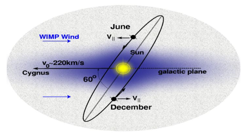
As our Solar System orbits around the galactic centre, it moves though this halo, experiencing an effective dark matter wind. This, combined with the tilt of the Earth's orbit around the sun, means we expect to see an annual modulation in the dark matter flux hitting the Earth. This modulation should have it's maximum around June when the Earth is moving into the wind, and it's minimum around December when it's moving away from the wind, regardless of location on Earth.
The current best candidate for dark matter are so-called Weakly Interacting Massive Particles (WIMPs). In direct detection experiments, we look at interactions between WIMPs and the nuclei in some target, such as Sodium Iodide (NaI) crystal. The WIMPs scatter elastically off nuclei in the target, and the recoil of the nuclei cause scintillation photons to be emitted, with summed energies of ~10keV range. Direct detection is hard, however, since WIMP interactions are rare events, where we expect << 1 count/day/kg. So identifying WIMP events, especially at low energies, requires significant background and noise suppression.
Various direct detection experiments (DAMA, CoGeNT, CRESST, CDMS, etc.) have already been run, but none yet have conclusively detected dark matter. Of particular interest from these experiments are the results from the DAMA/NaI and DAMA/LIBRA experiments. The DAMA experiments (Gran Sasso, Italy) ran direct detection using NaI(Tl) (Thallium doped Sodium Iodide) crystals, and observed an annual modulation in the 2-6keV energy region, which they claim is the result of the dark matter wind. However this interpretation is disputed. It is argued that the modulation could have come from some other unaccounted for signal – for example muon flux also has an annual modulation with peak around June (in the Northern Hemisphere).
DM-ICE is a joint venture between University of Sheffield (UK), and University of Wisconsin (Madison, USA). The aim, along with other independent direct detection experiments being run around the globe, is to test the DAMA result by looking for this same modulation, and by ruling out other possible sources of modulation. By running at the South Pole, DM-ICE is in the opposite hemisphere to DAMA, so seasonal effects – such as temperature and muon flux – are reversed, while the dark matter modulation should stays the same.
Context
For my final year project I was looking in particular at the performance stability of the detectors (loss of light yield, etc.) and how to correct the data for those effects. I also did some preliminary modulation analysis - looking for evidence of dark matter in the data.
This blog post isn't really to do with any of the work I did on my project, though. Rather, this is looking at how to remove noise from the data. For my project, this work had already been done, so I didn't have to worry about it. So why am I looking at noise removal now?
When the academic year was over, my project supervisor asked if I wanted to carry on working on the project (funded) for the summer. It made sense, since there was still work to do, and since I already knew the project well. So mostly I was doing more of what I did for the project. But the supervisor also wanted to adapt the DM-ICE project into a simplified version for groups of 3rd year students to do.
Specifically, the students would have to figure out the best cuts to remove noise, then do a modulation analysis to decide if there was evidence of dark matter.
So I set up a simplified version of the data and wrote up a description of the project for the students. The supervisor then asked if I'd work through the project and write up a model answer so that he'd have something to mark against. Hence, it was my turn to try the noise removal stuff.
Pulse Classification
In a DM-ICE detector, we have an 8.5kg NaI(Tl) crystal between paired photo-multipliers (PMTs). These two PMTs - DM0 and DM1 - record scintillation events as voltage pulses (in ADC units). When the raw data is processed, we look for pulses from both of the PMTs which occur within 100 ns of each other. These pairs of pulses are assumed to have come from the same scintillation event.
At low energies, pulses look something like this

where the various spikes represent single photo-electron events (SPE). Unfortunately, at low energies there is also a significant amount of noise events - specifically, electromagnetic interference (EMI) that look something like this

and 'thin peaks', that look something like this

So the task is to identify and remove these EMI and thin peak events.
From looking at plots of the pulses, it's fairly straightforward to tell the different event types apart. But computers can 'look' at the pulses. Instead, we have to define some parameter - values that we can calculate that will tell the computer something about the shapes of the pulses.
Take, for example, the EMI pulses. From the plot we can see that EMI pulses oscillate rapidly between positive and negative ADC values, where the SPE and thin peak events don't. So we can define some parameter, which we'll call 'emi', which basically counts how many times the pulse goes from positive to negative (or negative to positive) in the first 40 bins of the pulse.
So since the emi value is going to be much higher for EMI-type pulses than for SPE or thin peaks, identifying and removing EMI events is relatively easy.
Separating the SPEs from the thin peaks is less straightforward. For this, we calculate various other parameters - for example, since thin peaks will typically only have one peak, while an SPE event will have several, we can look at the peak number. Other things we can look at are how quickly the pulse decays to zero (log-meantime), or how the pulse energy is distributed. The details of how these parameters are calculated aren't important to this blog.
Human Learning
What you can do, then, is look at a bunch of pulses - plot it, what type of event is it? What are it's parameter values? You collect together the results and you ask, what sort of emi values do EMI-type events have? What sort of peak numbers do SPEs and thin peaks have. How can you use that information to tell the peaks apart?
And that's fine. But it's also boring. You have to plot, and calculate, and record. Repeat. Analyse. Boring.
I subscribe to the philosophy of "why do yourself what you can make a computer do?". In practice this usually means making the work more 'complicated' in the short term, but once it's done it makes life a whole lot easier. And while the work is more complicated, it's at least more interesting as well.
So what I did was I wrote a program. It looks something like this
 (I used Python with Numpy, Matplotlib for plotting, and PyQt4 for the GUI.)
Basically it plots the pulses and presents you with three buttons - signal (SPE), noise (thin peak), and EMI. On the front-end, all the user has to do is look at the plot and decide what type of event the pulse is. Meanwhile, on the back-end, the program calculates the parameters, and sorts them according to the user's classifications.
Once you've classified a set of pulses, you're presented with histograms of the different parameters, like this (for the emi value parameter)

where the different event types are plotted in different colours. This makes life a lot easier. For example, in the above, it's immediately apparent that EMI-type events can be removed from the data by cutting any event with an emi value above 25.
Machine Learning - Naive Bayes Classifiers
Lets make this more interesting. Sure, we can click through a bunch of peaks telling the program what's what. But wouldn't it be cooler if we could teach the program to tell the events apart itself?
Yes. Yes it would.
This is where machine learning comes in. Now there are various machine learning techniques, but the one I used in the program is called a 'Naive Bayes Classifier'. This is the sort of thing that's used in spam filters - it's a way of calculating, for example, what is the probability that a particular email is spam given that it mentions, say, penis enlargement or Nigerian princes.
Quick Introduction - Bayes' Theorem
Imagine there is a person. Sight unseen, what is the probability they are female? Well, given that there are roughly equal numbers of males and females in the world, the probability is about 50%. This is called the prior probability.
[Aside: in this example, we're assuming for simplicity that gender is a binary state.]
Now, we're given a new piece of information - this mystery person's height is 5'4 (five feet and four inches). Now the question is, what is the probability the mystery person is female, given they are 5'4? Well, females tend to be shorter than males (on average) so we might say that the mystery person is more likely to be female that male. But how do we quantify this new probability?
This is where Bayes' Theorem comes in. It looks like this
 Basically, this calculates the probability of a hypothesis (H) given some observation/evidence (O). p(H|O) is called the posterior probability.
For our example, we have the hypothesis "female" (F) and the observation "h=5'4". So the terms for this example are:
Putting it all together, we calculate the (posterior) probability of the mystery person being female given their height is 5'4, as

As we expected, this probability is much greater than 50% - the mystery person is more likely to be female than male, given their height.
*Aside: These figures come from average heights for Americans aged 20-80 for 2007-2008.
Obviously the probabilities would vary depending on where the mystery person is from, how old they are, etc. Since all we know about this mystery person is their height, we shouldn't really make assumptions about their background. But for the sake of demonstration (and convenience), these values are sufficient.
So how does this apply to noise removal?
Let's go back to EMI - we can ask, what is the probability that an event is EMI-type given it has an emi value of 30?
Using Bayes' Theorem, we have

Now we need to calculate the probabilities. We're going to assume we have a training set of (31) events that have already been classified. From this we can calculate/estimate these probabilities.
The prior, p(E), is pretty straightforward - what fraction of the events in the training set are EMI? This turns out to be around 22.6%
The probability of an EMI-type event having an emi value of 30 - p(emi=30|E) - is a little trickier to find. If our training set is small we may have no events with an emi value of exactly 30. But there could, at the same time, be several events with emi values slightly above or below 30.
Here then we have to make an assumption - we're going to assume that the distribution of emi values (for each event type) can be approximated by a normal distribution. This approach is called the 'Gaussian Naive Bayes', and is usually a reasonable approximation - if you look at the plot of emi values higher up, you'll see that they are roughly normally distributed.
So to find p(emi|E) we need to calculate the mean and standard deviation of the emi values for the EMI-type events in our training set. Obviously, when the training set is relatively small, the mean and standard deviation are going to have a large margin of error. So it's important to make sure we have a sufficiently large training set.
For p(emi=30|!E) - that is, the probability that an event that isn't EMI-type (signal or thin peak) has an emi value of 30 - we do the same procedure of calculating the mean and standard deviation of emi values for non-EMI events, again assuming a normal distribution.
For my training set of 31 events, the probability works out at p(E|emi=30) = 97.96%
In other words, an event with an emi value of 30 is almost certainly an EMI-type event.
For the full Naive Bayes Classifier, you just repeat the process above for all the parameters, then combine the probabilities. For example, the probability that an event is noise given its log-meantime value and peak number, would be given by

It's 'naive' because it assumes all the parameters are independent of each other. This isn't strictly true, but it's an acceptable approximation.
In fact, in practice, rather than calculating the probability, we calculate the 'log-likelihood ratio'

where Pi are the various parameters. From that it's pretty straightforward to extract the probability that an event is noise given its parameters. Alternatively, we can just say that if the log-likelihood is greater than 0 - if the probability of being noise is greater than the probability of being signal - then the pulse is classified as noise.
The point here is that, rather than investigating the differences between the different pulse types ourselves, then hard coding how to tell pulse types apart - e.g. explicitly writing in the code that an event is EMI-type if it has an emi value greater than 25, etc. - we instead show the code some examples of different pulses, and it 'learns' to tell the difference itself. This saves us a lot of work. In fact, we never even have to know what the differences between pulse parameters are.
When you're using the program, you can have it display what the algorithm thinks pulses are (and the associated probabilities). So you can click through a bunch of pulses, telling the algorithm what they are, and the algorithm will tell you what it thinks they are. As you 'teach' it, the algorithm will get better at telling the difference between pulses. And when you're happy with how well its classifications match up with your own, you can press a button and it will classify the rest of the pulses for you. How cool is that?
Finding the Best Cuts
Once the algorithms is adequately trained, we could just set it to work, going through the data, classifying and removing noise events. But for their project, the students aren't looking at machine learning, or statistics, or anything like that. Instead, they're asked to look for cutoff conditions for each of the parameters - for example, a pulse is noise if it has emi > 25.
To get a better idea of the problem we can look at our histograms of the parameters, with the different pulse type plotted in different colours. This is where the pulse classification comes in useful - the more pulses we classify, the clearer the distributions of parameters.
When you're looking at the emi values, as in the plot higher up, the cutoff is pretty easy - there's a clear gap between emi values for EMI-type pulses, and those for signal and thin peaks. For other parameters, the distinction is less clear, and often we have to make some trade off between leaving behind noise events and removing signal events. For example

Here, if you want to keep all the signal, you leave behind 23 (thin peak) noise events (34%). If you want to remove all the noise you end up also removing 6 signal events (54%).
Aside: Since EMI-type events are easily distinguished and removed with the emi value cut, they are not taken into account when we look at cuts for the other parameters, which are meant to separate signal from thin peaks.
So the question is, how can we determine the 'best' cuts?
This is basically an optimisation problem - we want to find the cut for which the maximum amount of noise AND the minimum amount of signal is removed. To do this, we need to come up with some metric/way of scoring how effective a given cut is, then we look for the cut that scores best.
We'll define Ni as the number of noise events and Si the number of signal events removed by some cut Ci. Because there are generally more noise events than signal, we're going to score based on the fractions of noise and signal removed - (Ni/N) and (Si/S) - where N and S are the total number of noise and signal events respectively. So the optimisation problem is finding the cut that gives (Ni/N) closest to one and (Si/S) closest to zero, simultaneously.
One approach to this optimisation is a 'nearest neighbour search'. To make this clearer, we can look at a scatter plot with points representing the fractions of signal and noise removed for different cuts. In this set-up, optimising means looking for the point that is nearest the bottom-right corner of the graph (1,0).

We can find the distance of each point from (1,0) using Pythagoras, making the scoring function
 which we want to minimise.
There is one caveat though - a cut that, for example, removes 10% of the signal and 60% of the noise will have the same distance score (0.41) as a cut that removes 40% of the signal and 90% of the noise. The latter removes more noise (almost all of it) but also removes more signal. In this case we have a choice - do we want to remove more noise, or save more signal?
To differentiate the two cases we can use the angle between the point and the noise-axis
 So if, for example, we want to save as much signal as possible then we want to minimise the angle. Or perhaps for a better balance between removing signal and noise, we should prefer the cut that gives an angle closest to 45deg. For myself, I prefer to save as much signal as possible. In practice, however, having two or more cuts with the same distance score is rare.
When it comes to reporting the (distance) scores, they are re-formatted as
 This gives a score of 1 for a cut that removes all noise and no signal, a score of -1 for a cut that removes all signal and no noise, a score of 0 for a cut that removes no signal or noise at all, etc. This score could be used in the optimisation algorithm (where it would need to be maximised), but the results would be the same, and the Pythagorean distance is easier to calculate.
Below is an example cut from this algorithm.
 Notice that it sacrifices one signal event for 15 noise events, but prefers to keep one more signal event, rather than removing an extra 5 noise events.
Ultimately, this technique of removing noise with parameter cutoffs is less effective than the Naive Bayes, largely because it considers all the parameters individually/independently. However, there are things called 'support vector machines' (SVM) which would probably be ideal for this problem. They look for a dividing 'line' between signal and noise, as above, but they consider all of the parameters together. OpenCV has an implementation of SVM, so I might give that a try at some point.
Last Word
As it started out, I just wanted to throw together a quick GUI to make my life easier, without worrying about error handling or bugs or any of that other fiddly stuff. Then I decided I wanted to try out some machine learning. And the more I worked on the program, the more features I thought of, and added.
So now, I have a program designed specifically for removing noise from DM-ICE data. But since DM-ICE has already had its noise removed (as far as possible), the program is basically of no use to anyone. Well, except maybe to any students working on this project. But that would be cheating - hence why I'm wary of posting the code.
Still, it was a fun little project.
Oatzy.
[Keep an eye out for news on DM-ICE.]
Background - Dark Matter and DM-ICE
According to current theories, dark matter makes up 23% of the mass-energy density of the universe. However, to date, it hasn't been conclusively observed directly. Instead, it's existence is inferred from large-scale gravitational effects, like the rotation curves of galaxies, and gravitational lensing. Based on rotation curves, we find that the outer edges of galaxies move as if there is more matter present than what we can directly observe. Consequently, it has been theorised that there is a halos of dark matter around the outer edges of galaxies, including our Milky Way.
As our Solar System orbits around the galactic centre, it moves though this halo, experiencing an effective dark matter wind. This, combined with the tilt of the Earth's orbit around the sun, means we expect to see an annual modulation in the dark matter flux hitting the Earth. This modulation should have it's maximum around June when the Earth is moving into the wind, and it's minimum around December when it's moving away from the wind, regardless of location on Earth.
The current best candidate for dark matter are so-called Weakly Interacting Massive Particles (WIMPs). In direct detection experiments, we look at interactions between WIMPs and the nuclei in some target, such as Sodium Iodide (NaI) crystal. The WIMPs scatter elastically off nuclei in the target, and the recoil of the nuclei cause scintillation photons to be emitted, with summed energies of ~10keV range. Direct detection is hard, however, since WIMP interactions are rare events, where we expect << 1 count/day/kg. So identifying WIMP events, especially at low energies, requires significant background and noise suppression.
Various direct detection experiments (DAMA, CoGeNT, CRESST, CDMS, etc.) have already been run, but none yet have conclusively detected dark matter. Of particular interest from these experiments are the results from the DAMA/NaI and DAMA/LIBRA experiments. The DAMA experiments (Gran Sasso, Italy) ran direct detection using NaI(Tl) (Thallium doped Sodium Iodide) crystals, and observed an annual modulation in the 2-6keV energy region, which they claim is the result of the dark matter wind. However this interpretation is disputed. It is argued that the modulation could have come from some other unaccounted for signal – for example muon flux also has an annual modulation with peak around June (in the Northern Hemisphere).
 |
| Source - ArXiv:0804.2741 |
Context
For my final year project I was looking in particular at the performance stability of the detectors (loss of light yield, etc.) and how to correct the data for those effects. I also did some preliminary modulation analysis - looking for evidence of dark matter in the data.
This blog post isn't really to do with any of the work I did on my project, though. Rather, this is looking at how to remove noise from the data. For my project, this work had already been done, so I didn't have to worry about it. So why am I looking at noise removal now?
When the academic year was over, my project supervisor asked if I wanted to carry on working on the project (funded) for the summer. It made sense, since there was still work to do, and since I already knew the project well. So mostly I was doing more of what I did for the project. But the supervisor also wanted to adapt the DM-ICE project into a simplified version for groups of 3rd year students to do.
Specifically, the students would have to figure out the best cuts to remove noise, then do a modulation analysis to decide if there was evidence of dark matter.
So I set up a simplified version of the data and wrote up a description of the project for the students. The supervisor then asked if I'd work through the project and write up a model answer so that he'd have something to mark against. Hence, it was my turn to try the noise removal stuff.
Pulse Classification
In a DM-ICE detector, we have an 8.5kg NaI(Tl) crystal between paired photo-multipliers (PMTs). These two PMTs - DM0 and DM1 - record scintillation events as voltage pulses (in ADC units). When the raw data is processed, we look for pulses from both of the PMTs which occur within 100 ns of each other. These pairs of pulses are assumed to have come from the same scintillation event.
At low energies, pulses look something like this
where the various spikes represent single photo-electron events (SPE). Unfortunately, at low energies there is also a significant amount of noise events - specifically, electromagnetic interference (EMI) that look something like this
and 'thin peaks', that look something like this
So the task is to identify and remove these EMI and thin peak events.
From looking at plots of the pulses, it's fairly straightforward to tell the different event types apart. But computers can 'look' at the pulses. Instead, we have to define some parameter - values that we can calculate that will tell the computer something about the shapes of the pulses.
Take, for example, the EMI pulses. From the plot we can see that EMI pulses oscillate rapidly between positive and negative ADC values, where the SPE and thin peak events don't. So we can define some parameter, which we'll call 'emi', which basically counts how many times the pulse goes from positive to negative (or negative to positive) in the first 40 bins of the pulse.
So since the emi value is going to be much higher for EMI-type pulses than for SPE or thin peaks, identifying and removing EMI events is relatively easy.
Separating the SPEs from the thin peaks is less straightforward. For this, we calculate various other parameters - for example, since thin peaks will typically only have one peak, while an SPE event will have several, we can look at the peak number. Other things we can look at are how quickly the pulse decays to zero (log-meantime), or how the pulse energy is distributed. The details of how these parameters are calculated aren't important to this blog.
Human Learning
What you can do, then, is look at a bunch of pulses - plot it, what type of event is it? What are it's parameter values? You collect together the results and you ask, what sort of emi values do EMI-type events have? What sort of peak numbers do SPEs and thin peaks have. How can you use that information to tell the peaks apart?
And that's fine. But it's also boring. You have to plot, and calculate, and record. Repeat. Analyse. Boring.
I subscribe to the philosophy of "why do yourself what you can make a computer do?". In practice this usually means making the work more 'complicated' in the short term, but once it's done it makes life a whole lot easier. And while the work is more complicated, it's at least more interesting as well.
So what I did was I wrote a program. It looks something like this
Basically it plots the pulses and presents you with three buttons - signal (SPE), noise (thin peak), and EMI. On the front-end, all the user has to do is look at the plot and decide what type of event the pulse is. Meanwhile, on the back-end, the program calculates the parameters, and sorts them according to the user's classifications.
Once you've classified a set of pulses, you're presented with histograms of the different parameters, like this (for the emi value parameter)
where the different event types are plotted in different colours. This makes life a lot easier. For example, in the above, it's immediately apparent that EMI-type events can be removed from the data by cutting any event with an emi value above 25.
Machine Learning - Naive Bayes Classifiers
Lets make this more interesting. Sure, we can click through a bunch of peaks telling the program what's what. But wouldn't it be cooler if we could teach the program to tell the events apart itself?
Yes. Yes it would.
This is where machine learning comes in. Now there are various machine learning techniques, but the one I used in the program is called a 'Naive Bayes Classifier'. This is the sort of thing that's used in spam filters - it's a way of calculating, for example, what is the probability that a particular email is spam given that it mentions, say, penis enlargement or Nigerian princes.
Quick Introduction - Bayes' Theorem
Imagine there is a person. Sight unseen, what is the probability they are female? Well, given that there are roughly equal numbers of males and females in the world, the probability is about 50%. This is called the prior probability.
[Aside: in this example, we're assuming for simplicity that gender is a binary state.]
Now, we're given a new piece of information - this mystery person's height is 5'4 (five feet and four inches). Now the question is, what is the probability the mystery person is female, given they are 5'4? Well, females tend to be shorter than males (on average) so we might say that the mystery person is more likely to be female that male. But how do we quantify this new probability?
This is where Bayes' Theorem comes in. It looks like this
For our example, we have the hypothesis "female" (F) and the observation "h=5'4". So the terms for this example are:
- p(F) - The probability of a person being female. This is our prior. [ 50% ]
- p(h=5'4|F) - The probability of a person being 5'4 given they are female. Or to put it more plainly, the probability of a female being 5'4. [ ~15.1% ]*
- p(h=5'4) - The probability of any person being 5'4. This can be calculated as the (weighted) average of the probabilities of a female being 5'4, and a male being 5'4. In other words, the probability can be expanded as
p(h=5'4) = p(h=5'4|F) p(F) + p(h=5'4|M) p(M)
where p(h=5'4|M) is the probability of a male being 5'4 [ ~1.8% ]*
Putting it all together, we calculate the (posterior) probability of the mystery person being female given their height is 5'4, as
As we expected, this probability is much greater than 50% - the mystery person is more likely to be female than male, given their height.
*Aside: These figures come from average heights for Americans aged 20-80 for 2007-2008.
Obviously the probabilities would vary depending on where the mystery person is from, how old they are, etc. Since all we know about this mystery person is their height, we shouldn't really make assumptions about their background. But for the sake of demonstration (and convenience), these values are sufficient.
Gaussian Naive Bayes - When the Training Set is Small
So how does this apply to noise removal?
Let's go back to EMI - we can ask, what is the probability that an event is EMI-type given it has an emi value of 30?
Using Bayes' Theorem, we have
Now we need to calculate the probabilities. We're going to assume we have a training set of (31) events that have already been classified. From this we can calculate/estimate these probabilities.
The prior, p(E), is pretty straightforward - what fraction of the events in the training set are EMI? This turns out to be around 22.6%
The probability of an EMI-type event having an emi value of 30 - p(emi=30|E) - is a little trickier to find. If our training set is small we may have no events with an emi value of exactly 30. But there could, at the same time, be several events with emi values slightly above or below 30.
Here then we have to make an assumption - we're going to assume that the distribution of emi values (for each event type) can be approximated by a normal distribution. This approach is called the 'Gaussian Naive Bayes', and is usually a reasonable approximation - if you look at the plot of emi values higher up, you'll see that they are roughly normally distributed.
So to find p(emi|E) we need to calculate the mean and standard deviation of the emi values for the EMI-type events in our training set. Obviously, when the training set is relatively small, the mean and standard deviation are going to have a large margin of error. So it's important to make sure we have a sufficiently large training set.
For p(emi=30|!E) - that is, the probability that an event that isn't EMI-type (signal or thin peak) has an emi value of 30 - we do the same procedure of calculating the mean and standard deviation of emi values for non-EMI events, again assuming a normal distribution.
For my training set of 31 events, the probability works out at p(E|emi=30) = 97.96%
In other words, an event with an emi value of 30 is almost certainly an EMI-type event.
Machine Peak Classification
For the full Naive Bayes Classifier, you just repeat the process above for all the parameters, then combine the probabilities. For example, the probability that an event is noise given its log-meantime value and peak number, would be given by
It's 'naive' because it assumes all the parameters are independent of each other. This isn't strictly true, but it's an acceptable approximation.
In fact, in practice, rather than calculating the probability, we calculate the 'log-likelihood ratio'
where Pi are the various parameters. From that it's pretty straightforward to extract the probability that an event is noise given its parameters. Alternatively, we can just say that if the log-likelihood is greater than 0 - if the probability of being noise is greater than the probability of being signal - then the pulse is classified as noise.
The point here is that, rather than investigating the differences between the different pulse types ourselves, then hard coding how to tell pulse types apart - e.g. explicitly writing in the code that an event is EMI-type if it has an emi value greater than 25, etc. - we instead show the code some examples of different pulses, and it 'learns' to tell the difference itself. This saves us a lot of work. In fact, we never even have to know what the differences between pulse parameters are.
When you're using the program, you can have it display what the algorithm thinks pulses are (and the associated probabilities). So you can click through a bunch of pulses, telling the algorithm what they are, and the algorithm will tell you what it thinks they are. As you 'teach' it, the algorithm will get better at telling the difference between pulses. And when you're happy with how well its classifications match up with your own, you can press a button and it will classify the rest of the pulses for you. How cool is that?
Finding the Best Cuts
Once the algorithms is adequately trained, we could just set it to work, going through the data, classifying and removing noise events. But for their project, the students aren't looking at machine learning, or statistics, or anything like that. Instead, they're asked to look for cutoff conditions for each of the parameters - for example, a pulse is noise if it has emi > 25.
To get a better idea of the problem we can look at our histograms of the parameters, with the different pulse type plotted in different colours. This is where the pulse classification comes in useful - the more pulses we classify, the clearer the distributions of parameters.
When you're looking at the emi values, as in the plot higher up, the cutoff is pretty easy - there's a clear gap between emi values for EMI-type pulses, and those for signal and thin peaks. For other parameters, the distinction is less clear, and often we have to make some trade off between leaving behind noise events and removing signal events. For example
Here, if you want to keep all the signal, you leave behind 23 (thin peak) noise events (34%). If you want to remove all the noise you end up also removing 6 signal events (54%).
Aside: Since EMI-type events are easily distinguished and removed with the emi value cut, they are not taken into account when we look at cuts for the other parameters, which are meant to separate signal from thin peaks.
So the question is, how can we determine the 'best' cuts?
This is basically an optimisation problem - we want to find the cut for which the maximum amount of noise AND the minimum amount of signal is removed. To do this, we need to come up with some metric/way of scoring how effective a given cut is, then we look for the cut that scores best.
We'll define Ni as the number of noise events and Si the number of signal events removed by some cut Ci. Because there are generally more noise events than signal, we're going to score based on the fractions of noise and signal removed - (Ni/N) and (Si/S) - where N and S are the total number of noise and signal events respectively. So the optimisation problem is finding the cut that gives (Ni/N) closest to one and (Si/S) closest to zero, simultaneously.
One approach to this optimisation is a 'nearest neighbour search'. To make this clearer, we can look at a scatter plot with points representing the fractions of signal and noise removed for different cuts. In this set-up, optimising means looking for the point that is nearest the bottom-right corner of the graph (1,0).
We can find the distance of each point from (1,0) using Pythagoras, making the scoring function
There is one caveat though - a cut that, for example, removes 10% of the signal and 60% of the noise will have the same distance score (0.41) as a cut that removes 40% of the signal and 90% of the noise. The latter removes more noise (almost all of it) but also removes more signal. In this case we have a choice - do we want to remove more noise, or save more signal?
To differentiate the two cases we can use the angle between the point and the noise-axis
When it comes to reporting the (distance) scores, they are re-formatted as
Below is an example cut from this algorithm.
Ultimately, this technique of removing noise with parameter cutoffs is less effective than the Naive Bayes, largely because it considers all the parameters individually/independently. However, there are things called 'support vector machines' (SVM) which would probably be ideal for this problem. They look for a dividing 'line' between signal and noise, as above, but they consider all of the parameters together. OpenCV has an implementation of SVM, so I might give that a try at some point.
Last Word
As it started out, I just wanted to throw together a quick GUI to make my life easier, without worrying about error handling or bugs or any of that other fiddly stuff. Then I decided I wanted to try out some machine learning. And the more I worked on the program, the more features I thought of, and added.
So now, I have a program designed specifically for removing noise from DM-ICE data. But since DM-ICE has already had its noise removed (as far as possible), the program is basically of no use to anyone. Well, except maybe to any students working on this project. But that would be cheating - hence why I'm wary of posting the code.
Still, it was a fun little project.
Oatzy.
[Keep an eye out for news on DM-ICE.]
Monday, July 02, 2012
Sharing a Burger Between Three
There are several ways to divide a burger evenly between three people.
Probably the best is to cut it radially (like a pizza). It can be tricky working out exactly where to make the cuts, but if you can pull it off, then all the pieces will be roughly identical (topping distribution notwithstanding).
But for the sake of arguing, lets say you want to divide the burger by making two parallel cuts: Where, then, do you make the cuts so that all three people get the same amount of burger?
NB/ This gets quite maths-heavy, so if you're not interested in that sort of thing, feel free to skip right to the end for the solution.
Geometry
For simplicity, we're going to consider the burger as a circle, and make the cuts so that each chunk has the same area. The two cuts are going to be the same distance from, and parallel to, the central axis of the burger, so we only need to consider the position of one of the cuts.
Here's the set-up
 We work out the area of the cut-off as the area of the circular segment, minus the area of the triangle.
- Aside: Radians
Radians are basically an alternative way of measuring angles. For maths and physics they're generally more useful than degrees.
They're relatively easy - there are 2pi radians in a full circle, so 2pi radians = 360 degrees
1 radian = 180/pi = 57.3 degrees
1 degree = pi/180 = 0.017 radians, etc.
Back to the circle; with angle x in radians, the area of the circular segment is
 The area of a triangle is half base times height..
- Aside: Area of the Triangle
We start by splitting the triangle down the middle, so that we have two identical right angle triangles
 The height, l = r*cos(x/2)
The base, b = 2*(r*sin(x/2))
So the area of the triangle is (l*b)/2 = r^2 sin(x/2)cos(x/2)
Finally, use the identity sin(2x) = 2sin(x)cos(x)
to get

So the area of the cut-off is
 and it needs to equal a third the area of the circle = 1/3 pi r^2.
So first, we need to find x satisfying
 or
or
 Once we have a value for x, we find where to make the cut from

Intermission
The thing about this equation is it doesn't have an exact, analytical solution - to find the solution you have to use numerical methods. Well, I say you have to use numerical methods; these days you can just type the equation into WolframAlpha, and you'll get a solution like *snaps fingers*
Which is nice. I even have the WolframAlpha app on my phone. But when I thought up this question I was on holiday in Sherwood forest, where there was literally no mobile singal.
So that was out of the question. And since I'm not in the habit of carrying a scientific calculator around with me, I was stuck with the basic calculator on my phone. It looks like this:
 No trig functions, no square roots, no pi button. It doesn't even do brackets, or have a memory function. Luckily, I am in the habit of carrying around a notepad and pen.
Anyway, there are two ways of working this out with only a basic calculator. The first is 'easier', but only if you know some stuff, and the numbers happen to be nice (in this case, they kind of are). The second is harder, in that it requires more number crunching, but it'll work with any numbers, and can be more precise.
Again, feel free to skip to the solution if you're not interested in the gritty details.
Method One
First of all, here's a graph of the two sides of the equation
We want to find the point at which the two graphs cross. We can see that that happens somewhere between 2pi/3 and pi (120 and 180 degrees). So, lets make a guess that it's exactly halfway between these two values: 5pi/6 (150 degrees).
For the right hand side of the equation: 5pi/6 - 2pi/3 = 0.52
NB/ I'm using pi=3.1416 (rounded to 4 decimal places). If you prefer, you could use the approximation 22/7. The result should be roughly the same.
For the left hand side of the equation, we need to work out sin(5pi/6)
At A-level, we were expected to memorise sin() and cos() of angles 0, 30, 45, 60, 90, and 180 (degrees). We were also expected to know the formulas for sin() and cos() of sums of angles. For sin(), it works like
 Why is this important? Well 150 degrees = 180 - 30 (5pi/6 rads = pi - pi/6)
So
 And since 0.5 is pretty close to 0.52 - less than 5% error - we can accept the convenience of that answer and say it's close enough.
So our approximate value of x is 5pi/6 = 2.618
[Incidentally, the identity for sin(2x) is just a special case of the above, with a=b=x; i.e. sin(2x) = sin(x+x) = 2sin(x)cos(x)]
Now we just need to work out l/r = cos(x/2) = cos(5pi/12)
For this one, 5pi/12 rads = 75 degrees = 45 + 30, so we can use
 So
So
 And we just have to evaluate that. But we don't have a square root button. Now, I just happen to know that sqrt(3) ~ 1.73 and sqrt(2) ~ 1.41.
But I'm just weird like that. Let's say you don't. How do you work it out?
- Aside: Square Roots
There are several ways of working out square roots with just basic operators. For two easy examples:
The first is 'Trial and Improvement' - pick a number, square it, does that give the right answer? If not, pick another number based on whether the last guess was too big or too small.
For example: sqrt(3)
The second method is the "Babylonian Method". It's more systematic, and can converge to the correct answer quicker than guessing. But it can be irritating if your calculator doesn't have a memory function.
It uses the recurrence relation
 Basically, you make a guess xn. Divide the number you want to square root (S) by xn. If xn is lower than the actual square root, then S/xn will be greater than it. That means the actual root will be between xn and S/xn, so we make the next guess xn+1 the average of these two values. Repeat until x is sufficiently accurate.
For example: sqrt(2)
Whatever way you do it, you repeat the process until you get the degree of accuracy you're happy with.
You should get the answer around l/r = 0.259
Method Two
We go back to the equation sin(x) = x - 2pi/3
We still have to find the solution numerically, we still don't have a calculator with a sin() function, and this time the numbers don't work out nicely.
So, the question is, how do we calculate sin(x)?
- Aside: Taylor Expansion
The Taylor Expansion of a function is a way of fitting a polynomial (sums of powers) to a more complicated function. It works like this
 Basically, it gives a way of converting a function we can't calculate into an infinite sum of powers of x, which we can calculate.
It's usually expanded around the origin (x0=0), since the equations work out neater. But you can do it around any point, x0=a. This is useful if the value you are trying to calculate is far from x=0. The closer x is to x0=a, the quicker the sum converges.
Even though the expansion is an infinite sum, it's usually sufficient to just take the first few terms, since each additional term makes a smaller and smaller contribution to the sum.
So the trick is working out how many terms you need to include to get some desired level of accuracy.
In this case, I'm going to use the Taylor Expansion of sin(x) around x0=pi, since the approximate value (2.6) is nearer to pi than 0.
Here's what the expansion looks like

So, how many terms do we need to include?
Here's what the graph looks like for different numbers of terms
For a value around 2.6, it can be shown that including the first two terms is correct to ~3 decimal places; the first three terms is correct to ~5 decimal places; the first four terms to ~7 decimal places, etc.
So I would probably go to the third term (for 5dp), but only take the result to 3dp.
NB/ We shouldn't get too hung up on getting an extremely accurate value for x, since we're already getting rounding errors from the factors of pi in the expansion. Also, since we're calculating x to 5dp, we should use pi=3.14159
That means we want to solve
 which can't be solved exactly.
So, for finding the correct value (without WolframAlpha), we can use any root-finding method. For what it's worth, I used Trial and Improvement; the other methods are easier with a computer.
But, note that the function is decreasing
 So if the guess gives a value greater than zero, you need to increase the value of x (and vice versa).
If you run through all that (I won't go into detail), it gives a value around x=2.605
Alternatively, you could expand around x0=5pi/6 (if you know/can work-out sin and cos of 150 deg without a calculator).
In this case you'd only need up to the term in x^2 (correct to ~4dp). Using this expansion would mean solving a quadratic equation, which is easy. But using this expansion can introduce more rounding errors from the factors of sqrt(3). It's a matter of preference, I guess. The answer should be about the same.
Finally, we need to calculate cos(x/2)
Again, we use the Taylor Expansion to calculate cos(). In this case, we're doing the expansion around x0=0; the expansion is
 In this case, you just keep adding terms until the result remains approximately constant to some desired degree of accuracy (3pd).
This gives a value around l/r = 0.265
So What is the Real Answer?
Once I got to somewhere where I could get at WolframAlpha, I checked the real numbers; here are the results:
 The approximation of x from Method One (2.618) is an over estimate by ~0.5%, which is relatively acceptable. The approximation from Method Two (2.605) is correct to 3 decimal places, which is definitely acceptable.
And for the value of l/r
 From Method One (0.259), the approximation is an under estimate by 2%, and correct to 2 decimal places, so is probably acceptable. The approximation from Method Two (0.265) is, again, correct to 3 decimal places. So that is also acceptable.
So, if the numbers happen to be convenient and you know some trigonometry, you're probably as well using Method One. If not, or if you just want more accuracy, then go for Method Two.
Applying the Results
The results are actually quite nice, in terms of practical application (dividing up a burger). The ratio of the radius (0.265) being close to one quarter, you find the cuts like this
 That is, find the central axis, then find the (imaginary) line halfway between the centre and the edge - make the cut halfway between the centre and this imaginary line (maybe cut an extra hair's breadth towards the edge). Repeat on the other side.
Easy.
So, now you know. Obviously, all this applies to dividing any circular thing evenly between three people. You could probably even adapt the methods for sharing between even more people.
And in theory, You could do all this with just pen and paper (no calculator). Though you probably wouldn't want to. I know I wouldn't..
Oatzy.
[Wow, I really managed to stretch that one out.]
Probably the best is to cut it radially (like a pizza). It can be tricky working out exactly where to make the cuts, but if you can pull it off, then all the pieces will be roughly identical (topping distribution notwithstanding).
But for the sake of arguing, lets say you want to divide the burger by making two parallel cuts: Where, then, do you make the cuts so that all three people get the same amount of burger?
NB/ This gets quite maths-heavy, so if you're not interested in that sort of thing, feel free to skip right to the end for the solution.
Geometry
For simplicity, we're going to consider the burger as a circle, and make the cuts so that each chunk has the same area. The two cuts are going to be the same distance from, and parallel to, the central axis of the burger, so we only need to consider the position of one of the cuts.
Here's the set-up

- Aside: Radians
Radians are basically an alternative way of measuring angles. For maths and physics they're generally more useful than degrees.
They're relatively easy - there are 2pi radians in a full circle, so 2pi radians = 360 degrees
1 radian = 180/pi = 57.3 degrees
1 degree = pi/180 = 0.017 radians, etc.
* * *
Back to the circle; with angle x in radians, the area of the circular segment is
- Aside: Area of the Triangle
We start by splitting the triangle down the middle, so that we have two identical right angle triangles

The base, b = 2*(r*sin(x/2))
So the area of the triangle is (l*b)/2 = r^2 sin(x/2)cos(x/2)
Finally, use the identity sin(2x) = 2sin(x)cos(x)
to get
* * *
So the area of the cut-off is
So first, we need to find x satisfying
Intermission
The thing about this equation is it doesn't have an exact, analytical solution - to find the solution you have to use numerical methods. Well, I say you have to use numerical methods; these days you can just type the equation into WolframAlpha, and you'll get a solution like *snaps fingers*
Which is nice. I even have the WolframAlpha app on my phone. But when I thought up this question I was on holiday in Sherwood forest, where there was literally no mobile singal.
So that was out of the question. And since I'm not in the habit of carrying a scientific calculator around with me, I was stuck with the basic calculator on my phone. It looks like this:

Anyway, there are two ways of working this out with only a basic calculator. The first is 'easier', but only if you know some stuff, and the numbers happen to be nice (in this case, they kind of are). The second is harder, in that it requires more number crunching, but it'll work with any numbers, and can be more precise.
Again, feel free to skip to the solution if you're not interested in the gritty details.
Method One
First of all, here's a graph of the two sides of the equation
 |
| hand-drawn with Skitch |
For the right hand side of the equation: 5pi/6 - 2pi/3 = 0.52
NB/ I'm using pi=3.1416 (rounded to 4 decimal places). If you prefer, you could use the approximation 22/7. The result should be roughly the same.
For the left hand side of the equation, we need to work out sin(5pi/6)
At A-level, we were expected to memorise sin() and cos() of angles 0, 30, 45, 60, 90, and 180 (degrees). We were also expected to know the formulas for sin() and cos() of sums of angles. For sin(), it works like
So
So our approximate value of x is 5pi/6 = 2.618
[Incidentally, the identity for sin(2x) is just a special case of the above, with a=b=x; i.e. sin(2x) = sin(x+x) = 2sin(x)cos(x)]
Now we just need to work out l/r = cos(x/2) = cos(5pi/12)
For this one, 5pi/12 rads = 75 degrees = 45 + 30, so we can use
But I'm just weird like that. Let's say you don't. How do you work it out?
- Aside: Square Roots
There are several ways of working out square roots with just basic operators. For two easy examples:
The first is 'Trial and Improvement' - pick a number, square it, does that give the right answer? If not, pick another number based on whether the last guess was too big or too small.
For example: sqrt(3)
1.5 -> 2.25 -> too small
1.7 -> 2.89 -> too small
1.8 -> 3.24 -> too big
1.75 -> 3.0625 -> too big
1.73 -> 2.9929 -> too small
1.74 -> 3.0276 -> too big
1.735 -> 3.010225 -> too big
1.7325 -> 3.00155625 -> too big
1.732 -> 2.999824 -> too small
etc.
The second method is the "Babylonian Method". It's more systematic, and can converge to the correct answer quicker than guessing. But it can be irritating if your calculator doesn't have a memory function.
It uses the recurrence relation
For example: sqrt(2)
x0 = 1.5 -> 2/1.5 = 1.33
x1 = (1.5 + 1.33)/2 = 1.4166.. -> 2/1.4167 = 1.41176..
x2 = (1.4167 + 1.41176..)/2 = 1.41421.. -> 2/1.41421 = 1.41421..
* * *
Whatever way you do it, you repeat the process until you get the degree of accuracy you're happy with.
You should get the answer around l/r = 0.259
Method Two
We go back to the equation sin(x) = x - 2pi/3
We still have to find the solution numerically, we still don't have a calculator with a sin() function, and this time the numbers don't work out nicely.
So, the question is, how do we calculate sin(x)?
- Aside: Taylor Expansion
The Taylor Expansion of a function is a way of fitting a polynomial (sums of powers) to a more complicated function. It works like this
It's usually expanded around the origin (x0=0), since the equations work out neater. But you can do it around any point, x0=a. This is useful if the value you are trying to calculate is far from x=0. The closer x is to x0=a, the quicker the sum converges.
Even though the expansion is an infinite sum, it's usually sufficient to just take the first few terms, since each additional term makes a smaller and smaller contribution to the sum.
So the trick is working out how many terms you need to include to get some desired level of accuracy.
* * *
In this case, I'm going to use the Taylor Expansion of sin(x) around x0=pi, since the approximate value (2.6) is nearer to pi than 0.
Here's what the expansion looks like
So, how many terms do we need to include?
Here's what the graph looks like for different numbers of terms
 |
| plotted with WolframAlpha |
So I would probably go to the third term (for 5dp), but only take the result to 3dp.
NB/ We shouldn't get too hung up on getting an extremely accurate value for x, since we're already getting rounding errors from the factors of pi in the expansion. Also, since we're calculating x to 5dp, we should use pi=3.14159
That means we want to solve
So, for finding the correct value (without WolframAlpha), we can use any root-finding method. For what it's worth, I used Trial and Improvement; the other methods are easier with a computer.
But, note that the function is decreasing
If you run through all that (I won't go into detail), it gives a value around x=2.605
Alternatively, you could expand around x0=5pi/6 (if you know/can work-out sin and cos of 150 deg without a calculator).
In this case you'd only need up to the term in x^2 (correct to ~4dp). Using this expansion would mean solving a quadratic equation, which is easy. But using this expansion can introduce more rounding errors from the factors of sqrt(3). It's a matter of preference, I guess. The answer should be about the same.
Finally, we need to calculate cos(x/2)
Again, we use the Taylor Expansion to calculate cos(). In this case, we're doing the expansion around x0=0; the expansion is
This gives a value around l/r = 0.265
So What is the Real Answer?
Once I got to somewhere where I could get at WolframAlpha, I checked the real numbers; here are the results:
And for the value of l/r
So, if the numbers happen to be convenient and you know some trigonometry, you're probably as well using Method One. If not, or if you just want more accuracy, then go for Method Two.
Applying the Results
The results are actually quite nice, in terms of practical application (dividing up a burger). The ratio of the radius (0.265) being close to one quarter, you find the cuts like this

Easy.
So, now you know. Obviously, all this applies to dividing any circular thing evenly between three people. You could probably even adapt the methods for sharing between even more people.
And in theory, You could do all this with just pen and paper (no calculator). Though you probably wouldn't want to. I know I wouldn't..
Oatzy.
[Wow, I really managed to stretch that one out.]
Saturday, March 03, 2012
Where are the Carriages?
<rant>
So it's around 9am, and you're waiting for a train. The trains in your area are a bit scummy, but whatever, you can't drive, and you've got to get to work/uni somehow. It's pretty busy, what with it being 9am, and when the train finally pulls up.. it's a single carriage.
Now a single car has around 50 seats, and this train is packed tight, with people standing in the aisles and the doorways, being forced to get intimate. And with everyone on board the conductor can barely get through the door. There are clearly enough people on this train to fill two cars, with people still having to stand.
So what gives? You're pretty pissed about having to stand for half an hour, and you've been inadvertently touched by strangers in ways you're not comfortable with. So you get your complaining hat on, and you turn to the internet to unleash the fury.
The train company's website directs you to their Twitter feed, where a poor public relations person is taking a barrage of vitriol from other angry commuters, while doing their best to remain polite and professional.
Several other people have already made your complaint, but all they're getting in return is "Apologies we try to avoid this where possible", or that the short trains were "due to operational reasons". And that's not really a satisfying response. You're not even sure it means anything.
</rant>
So Where Are The Carriages?
Disclaimer: I have no idea how the train company actually operates. I just like to write blogs about applied maths.
Here's the setup - you're in charge of logistics for the train company. You have a fixed number of trains/cars, and, for each day, a list of services and expected numbers of passengers.
How do you apportion the carriages between the services?
Obviously, every service needs at least one car, and services with more passengers need more cars.
So if you had, for example, three services with 50, 100, and 150 passengers respectively, and 6 cars, then it's easy to divvy them up - one for the first, two for the second, and three for the third.
But in general, it won't be possible to divide up the cars exactly like that; so what do you do about remainders?
This is actually similar to the problem of apportioning parliamentary seats between states in the US.
Currently there are 435 seats in the House of Representatives, which need to be shared out between the 50 states according to each state's population - the idea being that each seat should represent roughly the same number of voters.
There are various methods for doing this, but I'm only going to go over two of them.
The Hamilton method
Hamilton's Method is the easiest and most intuitive.
Say you've got only two services - service A has 85 passengers, service B has 115 passengers (200 passengers total). And you happen to have 4 carriages - a total 200 seats. So seats for everyone! Except service A needs 1.7 cars, and service B needs 2.3 cars. And you can't divide a car into two chunks.
But for starters, you can give one car to service A (50 seats), and two to service B (100 seats). So what about the fourth? Regardless of which service you give it to, some people are going to end up having to stand. So what you want to do is minimise that number.
For service A, 35 people need a seat. For service B, 15 people need a seat. So it makes sense to give the last car to service A. 15 people still have to stand, but - short of building more cars - there's really nothing you can do about that.
This is also known as the largest remainder method.
What if the passenger numbers were 75 and 125? Well in that case, I guess it would have to be a judgement call.
Anyway, that's the basic idea of the Hamilton method - divide up the cars as far as you can, then give the remaining car(s) to the service(s) which 'need them most'.
Things get trickier when you're dealing with larger numbers of passengers and cars, but ultimately it's pretty straight-forward.
The Huntington-Hill Method
Where trains differ from apportioning of parliamentary seats, is that a carriage has a fixed capacity, whereas the number of people a seat can represent is free to change.
And this means that you won't encounter some of the 'quirks' that arise from the Hamilton method - such as the Alabama Paradox (where increasing the total number of seats can mean a state losing seats), or the Population Paradox (where increasing a state's population can result in that state losing seats).
[You won't encounter them, but they're worth mentioning 'cause they're pretty cool.]
Huntington-Hill's Method - the one currently used by the House of Representatives - is, generally, a more powerful method than Hamilton's, and isn't susceptible to the various paradoxes. Another benefit is that it can be set up to guarantee that each state will get at least one seat.
It works by assigning seats, one by one, based on each state's 'priority quotient' - itself based on the state's population, and a 'modified divisor' based on the number of seats already allocated to that state.
But one advantage Hamilton's Method has over HHM, is that it will always give each service its ideal number of cars, either rounded up of down to the nearest whole number. So if a service's ideal number is 3.67, then Hamilton's method will assign either 3 or 4 cars to that service.
HHM, on the other hand, can 'violate quota' - that is, it can result in a given service being assigned more or fewer cars than it's ideal number (e.g. the 3.67 service might end up with only 2 cars). But this problem only occurs when the number of cars is fixed prior to apportioning. And sadly, it usually is.
As an aside, it turns out it's impossible to find a 'perfect' method of apportioning - one with neither paradoxes nor quota violating. Incidentally, the mathematical theory surrounding voting is quite fascinating. You know, if you're into that sort of thing.
Unfortunately..
Either method would work perfectly well. The problem is, while rounding up or down to the nearest car may seem trivial, the 50 seats that that one car represents can be a significant gain/loss for a service.
The lack of precise information can cause problems as well. You can only estimate how many passengers a given service will have in advance, and if you under-estimate, people are gonna be pretty pissed.
And on top of that, the numbers have to be recalculated from time to time as passenger numbers change..
Basically, getting the number of cars right can be tricky.
Of course, this all assumes that Northern Rail (or whatever company) has enough carriages to adequately satisfy its needs in the first place. Some how I doubt that's the case.
So ideally, NR needs to work out how many cars it actually needs, and build them. But I can't see that happening. And even if it did happen, it'd probably mean higher fares. And fares are pretty bad as they are.
Really, though, NR could do with a complete makeover just in general, given how shitty it is. Seriously, you should see the difference between them and the London Midland service. Ridiculous.
Incidentally, I also have strong feelings about the buses; don't even get me started. Trams are alright though - one every 10mins, seldom short of seats, sufficient leg-room.. bliss.
tl;dr - Where are the carriages, then? As it turns out, it's probably just that they don't have enough to go around.
This is what we get for privatising the trains...
Oatzy.
[My complaining hat is a trilby. I like to look bad-ass while I'm complaining.]
So it's around 9am, and you're waiting for a train. The trains in your area are a bit scummy, but whatever, you can't drive, and you've got to get to work/uni somehow. It's pretty busy, what with it being 9am, and when the train finally pulls up.. it's a single carriage.
Now a single car has around 50 seats, and this train is packed tight, with people standing in the aisles and the doorways, being forced to get intimate. And with everyone on board the conductor can barely get through the door. There are clearly enough people on this train to fill two cars, with people still having to stand.
So what gives? You're pretty pissed about having to stand for half an hour, and you've been inadvertently touched by strangers in ways you're not comfortable with. So you get your complaining hat on, and you turn to the internet to unleash the fury.
The train company's website directs you to their Twitter feed, where a poor public relations person is taking a barrage of vitriol from other angry commuters, while doing their best to remain polite and professional.
Several other people have already made your complaint, but all they're getting in return is "Apologies we try to avoid this where possible", or that the short trains were "due to operational reasons". And that's not really a satisfying response. You're not even sure it means anything.
</rant>
So Where Are The Carriages?
Disclaimer: I have no idea how the train company actually operates. I just like to write blogs about applied maths.
Here's the setup - you're in charge of logistics for the train company. You have a fixed number of trains/cars, and, for each day, a list of services and expected numbers of passengers.
How do you apportion the carriages between the services?
Obviously, every service needs at least one car, and services with more passengers need more cars.
So if you had, for example, three services with 50, 100, and 150 passengers respectively, and 6 cars, then it's easy to divvy them up - one for the first, two for the second, and three for the third.
But in general, it won't be possible to divide up the cars exactly like that; so what do you do about remainders?
This is actually similar to the problem of apportioning parliamentary seats between states in the US.
Currently there are 435 seats in the House of Representatives, which need to be shared out between the 50 states according to each state's population - the idea being that each seat should represent roughly the same number of voters.
There are various methods for doing this, but I'm only going to go over two of them.
The Hamilton method
Hamilton's Method is the easiest and most intuitive.
Say you've got only two services - service A has 85 passengers, service B has 115 passengers (200 passengers total). And you happen to have 4 carriages - a total 200 seats. So seats for everyone! Except service A needs 1.7 cars, and service B needs 2.3 cars. And you can't divide a car into two chunks.
But for starters, you can give one car to service A (50 seats), and two to service B (100 seats). So what about the fourth? Regardless of which service you give it to, some people are going to end up having to stand. So what you want to do is minimise that number.
For service A, 35 people need a seat. For service B, 15 people need a seat. So it makes sense to give the last car to service A. 15 people still have to stand, but - short of building more cars - there's really nothing you can do about that.
This is also known as the largest remainder method.
What if the passenger numbers were 75 and 125? Well in that case, I guess it would have to be a judgement call.
Anyway, that's the basic idea of the Hamilton method - divide up the cars as far as you can, then give the remaining car(s) to the service(s) which 'need them most'.
Things get trickier when you're dealing with larger numbers of passengers and cars, but ultimately it's pretty straight-forward.
The Huntington-Hill Method
Where trains differ from apportioning of parliamentary seats, is that a carriage has a fixed capacity, whereas the number of people a seat can represent is free to change.
And this means that you won't encounter some of the 'quirks' that arise from the Hamilton method - such as the Alabama Paradox (where increasing the total number of seats can mean a state losing seats), or the Population Paradox (where increasing a state's population can result in that state losing seats).
[You won't encounter them, but they're worth mentioning 'cause they're pretty cool.]
Huntington-Hill's Method - the one currently used by the House of Representatives - is, generally, a more powerful method than Hamilton's, and isn't susceptible to the various paradoxes. Another benefit is that it can be set up to guarantee that each state will get at least one seat.
It works by assigning seats, one by one, based on each state's 'priority quotient' - itself based on the state's population, and a 'modified divisor' based on the number of seats already allocated to that state.
But one advantage Hamilton's Method has over HHM, is that it will always give each service its ideal number of cars, either rounded up of down to the nearest whole number. So if a service's ideal number is 3.67, then Hamilton's method will assign either 3 or 4 cars to that service.
HHM, on the other hand, can 'violate quota' - that is, it can result in a given service being assigned more or fewer cars than it's ideal number (e.g. the 3.67 service might end up with only 2 cars). But this problem only occurs when the number of cars is fixed prior to apportioning. And sadly, it usually is.
As an aside, it turns out it's impossible to find a 'perfect' method of apportioning - one with neither paradoxes nor quota violating. Incidentally, the mathematical theory surrounding voting is quite fascinating. You know, if you're into that sort of thing.
Unfortunately..
Either method would work perfectly well. The problem is, while rounding up or down to the nearest car may seem trivial, the 50 seats that that one car represents can be a significant gain/loss for a service.
The lack of precise information can cause problems as well. You can only estimate how many passengers a given service will have in advance, and if you under-estimate, people are gonna be pretty pissed.
And on top of that, the numbers have to be recalculated from time to time as passenger numbers change..
Basically, getting the number of cars right can be tricky.
Of course, this all assumes that Northern Rail (or whatever company) has enough carriages to adequately satisfy its needs in the first place. Some how I doubt that's the case.
So ideally, NR needs to work out how many cars it actually needs, and build them. But I can't see that happening. And even if it did happen, it'd probably mean higher fares. And fares are pretty bad as they are.
Really, though, NR could do with a complete makeover just in general, given how shitty it is. Seriously, you should see the difference between them and the London Midland service. Ridiculous.
Incidentally, I also have strong feelings about the buses; don't even get me started. Trams are alright though - one every 10mins, seldom short of seats, sufficient leg-room.. bliss.
tl;dr - Where are the carriages, then? As it turns out, it's probably just that they don't have enough to go around.
This is what we get for privatising the trains...
Oatzy.
[My complaining hat is a trilby. I like to look bad-ass while I'm complaining.]
Subscribe to:
Posts (Atom)