Showing posts with label probability. Show all posts

Sunday, July 31, 2016

Barber Queue

Time was when I needed a hair cut, I'd go at noon on a weekday, when the barber's is typically empty. One of the perks of being unemployed.

But these days I have to get my haircuts on Saturdays, before noon. Which is bad enough in itself - ideally I'd never see Saturday mornings at all. And to make matters worse, Saturday morning is also when the barbers is at its busiest.

Hence, I found myself sat in the waiter area of a barbershop for the best part of an hour. But this got me thinking about how queuing works at a barbers.


First In Who's Next?

At its core, the barber's queue is just a first-in first-out (FIFO) queue. But it has two interesting features:


1) The queue 'structure' is unordered

In general the queue 'structure' will be a waiting area with a bunch of seats. When someone new joins the queue, they're free to sit wherever. In fact, odds are, they'll pick a seat in a similar way to how men choose urinals - attempting to maximise personal space.

But the key point is, if someone were to just look at the queue, they wouldn't be able to tell who was next.


2) Each member of the queue knows whether or not they're next

Each member of the queue probably doesn't know who exactly is next, but they do know (with reasonable certainty) whether or not it's them.

The way this works is relatively simple - when you join the queue, you're aware of who was there when you arrived (and of anyone who arrives after you). So when all the people who were there ahead of you have gone, you know that you're next.


O(M G)

Okay, lets break out some Python (2.7)

Just for fun, let's say that the capacity of the queue is fixed - i.e. the waiting area has a fixed number of seats (though in practice, people are free to stand, as I was forced to).

class BarberQueue(object):

    def __init__(self, capacity):
        self._capacity = capacity
        self._queue = [None]*capacity
        self._length = 0

    def __len__(self):
        return self._length

    def __str__(self):
        return ', '.join(str(i) if i is not None else '_'
                         for i in self._queue)

    def push(self, obj):
        pass

    def pop(self):
        pass

So each member of the queue has some awareness of who is ahead of them. But they don't need to know specifically who's who, they just need to keep track of how many are remaining. And in fact, that remaining count is exactly equivalent to the member's position in the queue.

class Member(object):

    def __init__(self, obj, position=0):
        self.value = obj
        self._position = position

    def __str__(self):
        return "%s (%s)" % (self.value, self._position)

    def is_next(self):
        return self._position == 0

    def move_up(self):
        self._position -= 1

So, going back to the push and pop methods

def push(self, obj):

    if self._length == self._capacity:
        raise Exception("Queue is full! Please come back later.")

    for i, m in enumerate(self._queue):
        if m is None:
            self._queue[i] = Member(obj, self._length)
            self._length += 1
            return

Here, we're picking a 'seat' by iterate over the queue looking for the first empty slot (with a value of None). We could implement any seat picking strategy we fancy, this is just the easiest.

Once we find an empty seat, we create a new 'Member' object for the item, with position set to the current length of the queue, then increment the queue length. Also, if the queue has no empty slots, we raise an exception.

def pop(self):
    if self._length == 0:
        raise Exception("The queue is empty")
    for i, m in enumerate(self._queue):
        if m is not None:
            if m.is_next():
                value = m.value
                self._queue[i] = None
                self._length -= 1
            else:
                m.move_up()
    return value

Here we iterate over the queue looking for the member who is 'next' (has position 0). While we're looking for the next person, we also de-increment the positions of the other members.

Of course, this isn't how things work in practice. The barber doesn't go to each person and say "are you next?", "how about you?". They simply say "who's next?", and the person who believes they are next steps forward. Though arguably, that's just equivalent to asking every member concurrently. But let's not complicate things.

>>> b = BarberQueue(3)
>>> for i in xrange(3):
 b.push(i)
 
>>> print b
0 (0), 1 (1), 2 (2)
>>> b.push(4)

Traceback (most recent call last):
  File "<pyshell>", line 1, in <module>
    b.push(4)
  File "<pyshell>", line 36, in push
    raise Exception("Queue is full! Please come back later")
Exception: Queue is full! Please come back later
>>> b.pop()
0
>>> print b
_, 1 (0), 2 (1)
>>> b.push(4)
>>> print b
4 (2), 1 (0), 2 (1)
>>> for _ in xrange(4):
 b.pop()
 
1
2
4

Traceback (most recent call last):
  File "<pyshell>", line 2, in <module>
    b.pop()
  File "<pyshell>", line 46, in pop
    raise Exception("Empty queue!")
Exception: Empty queue!
>>> print b
_, _, _

So there we have it. Of course, this type of queue isn't really useful from a programming perspective.

All of insertion, deletion, and lookup are worst-case \(O(N)\), where N is the queue's capacity (not the number of people in the queue). Which is pretty much worse than all other types of queue.


Why do items keep disappearing from my queue?

Okay, let's move away from computer-sciencey queues. There are certain behaviours in real-world queues that don't apply or wouldn't make sense to programmatic queues.

For one, as I alluded to earlier, the capacity of the queue is not enforced - there's room for overflow, even if it means people have to stand.

But on the other hand, when a place does get that full, people are less likely to stick around.

In particular, we have two situations:


1) There's a non-zero probability that a person will not stick around if the queue is full or close to full. This probability will tend to be related to the length of the queue when that person arrives

\[p(not join) \sim f(capacity, length)\]

For example,

\[p(not join) = A\left(\frac{length}{capacity}\right) - C\]

where A and C are some constants relating to how likely the person is to stick around if the queue is 'full', and at what point they consider the place to be 'too full'.


2) There's a non-zero probability that a person already in the queue will leave before they're served.  This probability will typically depend on how long the person has been waiting, and how many people are still ahead of them

\[p(leave) \sim g(wait, position)\]

It's interesting because as time passes, wait increases, but position decreases. So how the probability evolves depends on how those factors balance against one another.

In particular, the probability evolution will likely depend on how each particular person responds to the sunk-cost fallacy - i.e. are they the sort to think "well, I've waited this long, I might as well see it through to the end", or do they think "this is taking too long, I've got better things to do with my time"?

For the sake of arguing, lets go with an exponential function for the general form.

For a sunk-cost person we might have

\[p(leave) = B \cdot \exp\left(-d\cdot \frac{wait}{position}\right)\]

This is a function where p goes to zero as position goes to zero or wait goes to infinity (B and d are some arbitrary constants).

Whereas for a non-sunk-cost person we might have

\[p(leave) = B \cdot \exp\left(-\frac{d}{wait \cdot position}\right)\]

This is a function where p goes to zero as position goes to zero, but goes to one as wait goes to infinity.

This gives us an interesting graph

Because 'position' is discrete you get this nice step function, with intervals of the probability steadily rising, then suddenly dropping. We can also see that there's a point at which probability of leaving is maximum, around the time you're in the middle of the queue. Which seems plausible.


We also have situations where a person will leave and come back later. But since, when they come back, they have to join the back of the queue, they're mathematically indistinguishable from a someone arriving for the first time.


One other complicating situation is people in groups. For example, if there's a parent and child ahead of you in the queue, the child is getting their hair cut by one member of staff, the parent is waiting; another member of staff asks 'who's next?' - is it you or the parent?

Situations like these add uncertainty into a member's queue position, and by extension their knowledge of whether they're next.

In that situation, we might wait to see if anyone else steps up, and if not we can assume it's our turn.

So we have \(p(next)\), which is a Bayesian probability that updates over time to reflect whether anyone else has stepped up yet. The longer we wait with no-one stepping up, the closer our probability gets to one.
Of course, if you wait too long, someone behind you might assume you're not in the queue after all and try to go ahead of you. But that's a topic for another blog.


Nothing's so simple that it can't be made complex

I've written about queuing before, in the context of a mathematical model of a cafe.

The long and short of it is this - people arrive at random (following a Poisson distribution) and join the queue with some probability (see above). Each iteration, some people are served, some join the queue, some get tired of waiting and leave, etc.

I'm going to iterate in 5 min time-step and say that a haircut takes 10-25 minutes (i.e. 2-5 steps). The exact duration is randomly generated for each customer.

I'm going to say that on average one person shows up every 10 minutes (0.5 per step). Here's an example of how that might look over 12 steps (one hour), using the Poisson distribution: [2, 0, 2, 0, 0, 0, 1, 0, 0, 1, 0, 0]

I set up the simulation so that you specify some number of steps for the barbers to be considered 'open'. After that, no more people are added to the queue, but the simulation keeps running until the queue is empty.

To begin with, I made it so that everyone who arrived stayed.

With 2 workers, capacity 10, and an arrival rate of 0.5, the queue length typically stayed below 3. The highest I saw it go was 7, which is still comfortably within capacity.
Above is an example of how the queue size varied over time in a particular simulation.

Increasing the arrival rate to 0.7, the average maximum queue length goes up into the low teens. And when the rate goes up to 1, the maximum queue length goes all the way up into the 30s.

Homework question - how does maximum queue length vary as a function of number of workers and arrival rate?

As I mentioned, those simulations assumed that everyone stuck around. Once you turn on probabilistic leaving, things get a bit more interesting.

I tried both versions of the leaving probability. The result was largely the same, except that sunk-cost people tend to leave sooner - average wait before leaving 2.6 for sunk vs 7.4 for non-sunk. This is what we'd expect - people adhering to sunk cost will tend to leave before they get too invested.

In the above example, orange is a time step when someone left the queue, and red is when a newcomer decided not to join the queue. I tuned the probability constants so that people don't start leaving until we're close to or at capacity, as we'd expect in real life.


You and I have different ideas of what constitutes 'interesting'

Going back to the original description of the barber's queue, here's an example of a full queue (bracketed numbers are queue positions)

542b5af6 (3), 33e323cf (5), 69e60241 (6), b3f12010 (0), fc89732e (7), 991f8709 (1), a0cb93cc (2), 17186c75 (4), 57269a3e (8), 8f1b61ca (9)

Notice how, even with the basic seat picking strategy (take the first available), the members aren't in a predictable ordered.


When we look at the waiting times, we can see some interesting things. For example
...
1c7081d1 waited 7.0
34 1
35 3
50be68cf waited 9.0
36 3
37 4
26ca11b7 waited 3.0
38 3
39 3
a571a7da waited 5.0

...

Here we have a person who had to wait 9 steps (45mins) to be served, followed by someone who only had to wait 3 steps (15mins). Which just goes to show, how long you wait in a queue is very much a matter of timing and luck.


It's also interesting that you can run the simulation multiple times with the exact same settings, and one time the queue will never go higher than 4, while in the the next it'll go as high as 13. This is complexity at work - various small random factors in the model interacting to produce wildly different outcomes.


So yeah. If you're interested, you can see the full code here. I may have gotten carried away with the object-orienting.


Oatzy.


[Post-Script

My boss recently pointed out that it'd been over a year since my last blog post. That was another perk of being unemployed - more time to come up with dumb blog posts. Anyway, here's a quick update on some stuff.


Pirate Game

The last blog post was about the making of an Android game - The Pirate Game.

The game is now finished-ish and has been released in 'beta' on the Play Store.

In the previous post, I mentioned that the game would eventually get a less utilitarian design. I ended up making that design myself (because I'm a control freak). I'm pretty pleased with how it turned out.
Also, following a... less than positive review, I added some new game play modes.

I never did figure out multiplayer, though. If I ever get the time or inclination to go back to the game, that'll be on the todo list. But for the time being, I don't anticipate any updates to the game. Certainly not any time soon.


New Job

So yeah. I finally got a job. I'm now a Software Developer at a company called Pixit Media.

The company sells large scale 'storage solutions' to companies primarily in the VFX industry, as well as universities and other such people that do high performance computing.

What I personally work on is primarily a Python API for the IBM Spectrum Scale (GPFS) filesystem. You can see the API docs online. I wrote a decent amount of the documentation (and the code that's being documented).

In particular, the 'Getting Started With List Processing' guide. Admittedly the topic is a bit niche - I doubt many readers of this blog even know of GPFS, let along have a cluster with it installed. But you might still find it interesting; you can learn some stuff about MapReduce - a technique for taking advantage of parallelism when processing large data-sets.

There's also the 'example scripts' repository - scripts written to use the API, some of while I wrote. But, again, they're a bit niche.

]

Sunday, June 28, 2015

The Pirate Game

A few months ago, my friend was telling me about this mobile game he wanted to make. He, and some of our other friends, are teachers, and this is a game they play with their students. The students apparently love it. And if there were an app version, they'd be willing to pay 59p for it. Or so they say.

Now, as he was explaining the game to me, I thought maybe he was building towards asking for my help. I felt almost betrayed that he didn't. Several years ago, I'd built a website for this friend that he'd had nothing but praise and gratitude for.

A month or so later, I got a text message - "How are you at programming?" For whatever reason, the guy they had originally 'hired' wasn't doing it anymore.

"I'm capable", I replied. I'd done a course in Java at university. Admittedly, that was 'Java for Mathematicians'. And it was also almost 8 years ago. But how hard could it be to pick up again? Just like coding a bicycle. Or something like that...


The Game

As the title of the blog suggests, its called 'The Pirate Game'. In the classroom it's played on paper.

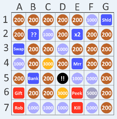
Basically, you have a 7x7 grid filled with items - mostly coins, but also some items that let you do other things. There are attacks that let you, for example, rob or kill other players. There's a shield and a mirror that let you defend against attacks. There's a bank item that let's you save whatever points you have from being stolen, etc. There's a bomb that blows you up (sets your points to zero). And so on.

This is the prototyping design. The final product will look less utilitarian.

At the start of the game, the players arrange the items in their grids to their liking. The teacher (game) then calls out random squares, and the players get whatever is in that square on their own grid. In the classroom, if a player gets an attack item, they have to raise their hand and tell the teacher who they want to use it on. The winner is whoever has the most points when all the squares have been called.


Making Games 1: The Right Tools

In a previous blog, I asserted that making mobile games was difficult. In fact, it turns out to not be so bad with the right framework. In this case I used the popular LibGdx. What's particularly nice about it is that there are a lot of how-to guides, and there's plenty of help for when things go wrong.

As they say, programming is 1% inspiration, 99% Googling.

For anyone interested in making their own Android game, I found these guides particularly helpful,

LibGdx Zombie Bird Tutorial
LibGdx Game Development Essentials
Set up Google Services with LibGdx


HAL9000

I got a first working version of the game done in the space of about a month - this was just the basic game mechanics, a bare-bones interface, and a single computer opponent that I could play against to check that the mechanics were doing what they were supposed to.

In those first few tests of the game, I found that the computer player kept beating me - at one point, 7 to 1. This seemed strange - neither I nor the computer could choose who we attacked, or which defences we used. So really, there wasn't anything either of us could do to influence the outcome of the game. The winner should have been totally random.

So loosing 7 times out of 8 seemed significant to me. As far as I could tell, the mechanics were working correctly. The only theory I could come up with was that maybe there was some advantage in the order in which we took our turns.

To try and figure out what was going on, I created a simulation. Basically, I re-wrote a very stripped down version of the player and game mechanics in Python. I then had two computer players play against each other in 10,000 matches. The results from this were - Player 1: 5005, Player 2: 4995.
In other words, the winner was just random chance. And turn order didn't matter.

If nothing else, this was a lesson in not drawing conclusions from such a small data set - it's not really statistically significant if there are only 8 data points (that's a standard error of ~3). After playing more games, the wins did end up averaging out.


Making Games 2: Coordinating Players

Development progressed. I got the full game mechanics working, and added more computer players (Clu and Ultron). I was now able to choose who I wanted to attack and what defences I wanted to use.

But the ultimate goal for the game is to let users play against their (human) friends. This meant I had to do a massive re-write to generalise the interaction mechanics.

Okay, lets look at an example of an interaction. Say I want to swap points with another player. First, my device needs to pop-up a player select dialog. Once I pick a target, the game needs to inform that player that I'm trying to swap points with them. If that player has a shield, their device needs to pop-up a dialog asking if they want to use it. The game then needs to inform me of my target's response - and if the target doesn't defend them self, we need to tell each other what our respective points are so that we can complete the swap.

That's a lot of back and forth to handle. Here are the rough diagrams I drew when I was trying to get the mechanics straight in my head.

I doubt this helps clarifies things for anyone else.

So the way the interaction works in the code is, the attacker sends their target a data object telling them who the attacker is, what attack they're trying to use, and what points they have (though the points aren't visible to the target). Once the target has chosen their defence, they complete their side of the attack processing - so in the swap example, if the target doesn't defend, they set their points to those of the attacker.

The target then sends the attacker's original data, along with the defence they chose (if any) and their (pre-attack) points to all the other players. If the recipient is the original attacker, they complete their side of the attack. Then, all players are shown a notification telling them what happened.
I figured I should give the computer players more piratical names.

All this coordination is done by a turn handler class. And what's nice is the computer players can also interact with each other, and with the local human player, via the turn handler.

All I need to do now is set up the stuff that actually sends the data between network players.


Game Theory

Through testing (looking for bugs and the like), I've played this game A LOT. And I've gotten a pretty good feel for how it works. It's actually quite fascinating when you really get into it. (Or maybe that's just Stockholm Syndrome talking).

Information is important to the game. Without it, players would be forced to make their moves at random. And when that happens, winning becomes mostly random chance. This is why players are shown notifications when other players interact - it allows them to strategise.

The most basic strategies are things like - rob people who have lots of points, don't try to rob people who have just been killed (they don't have any points to take), defend yourself when you have a lot of points (if you can). Really, this is just being sensible.

Then there are more subtle strategies. For example, sometimes it's better to lose a lot of points to the bomb or to being killed (removing those points from the game) rather than letting another player take them. Because, you don't need a lot of points to win, you just need more than everyone else.

Given the inherent randomness of the game, a lot of how you play will come down to how risk-averse you are. For example, a particularly risky strategy might be to let an opponent rob you (saving your defences), in the hopes that you can steal back your points, and more, later on.

When you play against humans (rather than AI), a whole bunch of social factors can come into play too. From what I hear, in the classroom, students tend to disproportionately target any members of staff that are playing. Though I can't imagine why.

One other interesting feature of the game is that it sometimes forces players to make disadvantageous moves. There's the bomb item that will take away your points when it inevitably comes up. And if you're in first place, the swap item forces you to give your points, and the lead, to another player.

So yeah, the game's not as simple as it might seem on the face of it.


Artificial Intelligence

In the first fully featured version of the game, the computer players made their decisions completely randomly. And that was fine - the game is perfectly playable with random opponents, it's not too easy, and the randoms can and will beat you on occasion. Sometimes by an embarrassing margin.

But random players also do things that don't make sense. So I wanted to create some computer players that used basic strategies to play more intelligently.

For interactions, these intelligent computer players (AI) use literal hit lists and avoid lists. As mentioned above, when two players interact, that information is sent to all other players. For humans, this information is displayed as a notification. For the AI, the information is processed to build/modify the hit and avoid lists.

For example, if Player 1 steals a lot of points from Player 2, then Player 1 is added to the hit list and Player 2 is added to the avoid list. If another player then kills Player 1, Player 1 is removed from the hit list and added to the avoid list. And so on.

If the AI then gets an attack square, they'll first check their hit list for a target. If the hit list is empty, they'll chose a random opponent who isn't on the avoid list. And so on.

There are also various basic heuristics for choosing which defences to use (and when), and for choosing a square when they get 'Choose Next'.

As they are, the AI are quite formidable, and at times frustratingly so. In general, I think it's better to have a mix of random and intelligent computer players. The AI offer a challenge, while the chaotic influence of the random players keeps things interesting.


Measuring Difficulty

In the game's current form, you can play against 2-7 computer players, and these players can be either random or 'intelligent' (as above).  That means 33 unique opponent set-ups. Which raises the question - how can we rate the difficulty of any given set-up. 

Obviously it's harder to win when there are more opponents. Specifically, the probability of a random player winning in a game of N random players is 1/N. Think of it like this - if all the players behave in the same way, they are indistinguishable. And if they're indistinguishable, they must all have the same probability of winning (turn order doesn't matter).

The same logic applies to intelligent computer players (AI) - since they all follow the same set of rules, they must also be indistinguishable from each other. Therefore, the odds of an AI winning in a game of N AI players must also be 1/N .

But what happens when there's a mix? How much harder are AI to beat than randoms?

To answer that, we can run some more simulations. This time, instead of re-writing code in Python, I created a modified version of the turn handler (see above) within the game project itself. Essentially I just removed all code that related to human players, and added a few bits to track statistics.

I set up the 33 different player configurations, ran 10,000 matches for each, and worked out the probability of winning for an AI player - for simplicity, we're assuming that a human player (playing strategically) is roughly equivalent to an AI.

From those simulations I made this lovely surface plot (using matplotlib).

Configurations with more than 7 opponents have been set to zero.

And what we find is AI are roughly twice as hard to beat as randoms - notice the surface is higher on the right hand side (when there are fewer AI).

In other words, your odds of winning in a match against two AI is roughly equal to your odds of winning in a match against four randoms. For simplicity, we're going to assume that the relationship is exactly two to one.

We can now calculate an approximation of the odds of winning as

\[ p(R, I) = \frac{2}{R + 2(I+1)} \]

And if we compare these probabilities to those from the simulations, we find that they are within standard error (order 0.01 for 10,000 trials).


To get a difficulty rating, we can just turn the probability on it's head, and normalise by the probability for the easiest set-up (2 random opponents). That is,

\[ D = \frac{p_0}{p} = \frac{R + 2(I+1)}{4} \]

This gives us a difficulty rating between 1 and 4, which lets us easily divide the difficulty into three levels - easy, medium, and hard. Though, if your odds of winning in the easiest possible game is only 50:50, can it really be considered 'easy'?

Another nice property of this difficulty rating system is that the difficulty ratios match the probability ratios - that is, your odds of winning a 2 are half your odds of winning a 1, and so on. Specifically, your odds of winning are roughly \( \frac{1}{2D} \)

Incidentally, if we assume our human player instead makes their moves completely at random, then their odds of winning are lower overall - \( p = \frac{1}{R+1+2I} \) - but the difficulty stratification works out the same.


Conclusion

Ordinarily, I'd include my code for this sort of thing. But in this case, doing so might undermine my (and my friends') income. And they very kindly told me that I'd get the majority of the profits. Whatever those may ultimately be.

So far we've made a whopping 7p (!) just from having adMob set up in the test builds.

But before we can make any (real) money, we have to actually finish the game. The single player version is mostly done, and should be released in the near future. The last big thing to do is the UI (which is someone else's problem job).

Then the hard part is going to be setting up multi-player with Google Play Services. In particular, because there aren't any good guides (that I can find) for setting up Google multi-player with LibGdx.

When it is done, I'll post links and such here for anyone that might be interested.

[edit] - If you want to try the current beta, you can get it here.

Also, given that making an Android game has turned out to be much easier than I expected, I may in fact make the previously discussed relativity game myself (once the Pirate Game is finished). In that case, I might also provide my code.


Oatzy.


[I'd love to make an AI that uses machine learning to counter human players' personal strategies.]

Tuesday, October 14, 2014

Dark Matter and Machine Learning

If you're a long time follower of this blog you'll probably have noticed I haven't posted much in the last two/three years. This is because I've been busy with university stuff. This blog is sort of related to that. The following section is an edited version of the background I wrote for my final year project report (hence why it's so formal). Enjoy.


Background - Dark Matter and DM-ICE

According to current theories, dark matter makes up 23% of the mass-energy density of the universe. However, to date, it hasn't been conclusively observed directly. Instead, it's existence is inferred from large-scale gravitational effects, like the rotation curves of galaxies, and gravitational lensing. Based on rotation curves, we find that the outer edges of galaxies move as if there is more matter present than what we can directly observe. Consequently, it has been theorised that there is a halos of dark matter around the outer edges of galaxies, including our Milky Way.


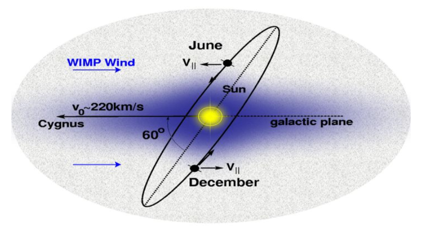
As our Solar System orbits around the galactic centre, it moves though this halo, experiencing an effective dark matter wind. This, combined with the tilt of the Earth's orbit around the sun, means we expect to see an annual modulation in the dark matter flux hitting the Earth. This modulation should have it's maximum around June when the Earth is moving into the wind, and it's minimum around December when it's moving away from the wind, regardless of location on Earth.

The current best candidate for dark matter are so-called Weakly Interacting Massive Particles (WIMPs). In direct detection experiments, we look at interactions between WIMPs and the nuclei in some target, such as Sodium Iodide (NaI) crystal. The WIMPs scatter elastically off nuclei in the target, and the recoil of the nuclei cause scintillation photons to be emitted, with summed energies of ~10keV range. Direct detection is hard, however, since WIMP interactions are rare events, where we expect << 1 count/day/kg. So identifying WIMP events, especially at low energies, requires significant background and noise suppression.

Various direct detection experiments (DAMA, CoGeNT, CRESST, CDMS, etc.) have already been run, but none yet have conclusively detected dark matter. Of particular interest from these experiments are the results from the DAMA/NaI and DAMA/LIBRA experiments. The DAMA experiments (Gran Sasso, Italy) ran direct detection using NaI(Tl) (Thallium doped Sodium Iodide) crystals, and observed an annual modulation in the 2-6keV energy region, which they claim is the result of the dark matter wind. However this interpretation is disputed. It is argued that the modulation could have come from some other unaccounted for signal – for example muon flux also has an annual modulation with peak around June (in the Northern Hemisphere).
Source - ArXiv:0804.2741
DM-ICE is a joint venture between University of Sheffield (UK), and University of Wisconsin (Madison, USA). The aim, along with other independent direct detection experiments being run around the globe, is to test the DAMA result by looking for this same modulation, and by ruling out other possible sources of modulation. By running at the South Pole, DM-ICE is in the opposite hemisphere to DAMA, so seasonal effects – such as temperature and muon flux – are reversed, while the dark matter modulation should stays the same.


Context

For my final year project I was looking in particular at the performance stability of the detectors (loss of light yield, etc.) and how to correct the data for those effects. I also did some preliminary modulation analysis - looking for evidence of dark matter in the data.

This blog post isn't really to do with any of the work I did on my project, though. Rather, this is looking at how to remove noise from the data. For my project, this work had already been done, so I didn't have to worry about it. So why am I looking at noise removal now?

When the academic year was over, my project supervisor asked if I wanted to carry on working on the project (funded) for the summer. It made sense, since there was still work to do, and since I already knew the project well. So mostly I was doing more of what I did for the project. But the supervisor also wanted to adapt the DM-ICE project into a simplified version for groups of 3rd year students to do.

Specifically, the students would have to figure out the best cuts to remove noise, then do a modulation analysis to decide if there was evidence of dark matter.

So I set up a simplified version of the data and wrote up a description of the project for the students. The supervisor then asked if I'd work through the project and write up a model answer so that he'd have something to mark against. Hence, it was my turn to try the noise removal stuff.


Pulse Classification

In a DM-ICE detector, we have an 8.5kg NaI(Tl) crystal between paired photo-multipliers (PMTs). These two PMTs - DM0 and DM1 - record scintillation events as voltage pulses (in ADC units). When the raw data is processed, we look for pulses from both of the PMTs which occur within 100 ns of each other. These pairs of pulses are assumed to have come from the same scintillation event.

At low energies, pulses look something like this


where the various spikes represent single photo-electron events (SPE). Unfortunately, at low energies there is also a significant amount of noise events - specifically, electromagnetic interference (EMI) that look something like this


and 'thin peaks', that look something like this


So the task is to identify and remove these EMI and thin peak events.

From looking at plots of the pulses, it's fairly straightforward to tell the different event types apart. But computers can 'look' at the pulses. Instead, we have to define some parameter - values that we can calculate that will tell the computer something about the shapes of the pulses.

Take, for example, the EMI pulses. From the plot we can see that EMI pulses oscillate rapidly between positive and negative ADC values, where the SPE and thin peak events don't. So we can define some parameter, which we'll call 'emi', which basically counts how many times the pulse goes from positive to negative (or negative to positive) in the first 40 bins of the pulse.

So since the emi value is going to be much higher for EMI-type pulses than for SPE or thin peaks, identifying and removing EMI events is relatively easy.

Separating the SPEs from the thin peaks is less straightforward. For this, we calculate various other parameters - for example, since thin peaks will typically only have one peak, while an SPE event will have several, we can look at the peak number. Other things we can look at are how quickly the pulse decays to zero (log-meantime), or how the pulse energy is distributed. The details of how these parameters are calculated aren't important to this blog.


Human Learning

What you can do, then, is look at a bunch of pulses - plot it, what type of event is it? What are it's parameter values? You collect together the results and you ask, what sort of emi values do EMI-type events have? What sort of peak numbers do SPEs and thin peaks have. How can you use that information to tell the peaks apart?

And that's fine. But it's also boring. You have to plot, and calculate, and record. Repeat. Analyse. Boring.

I subscribe to the philosophy of "why do yourself what you can make a computer do?". In practice this usually means making the work more 'complicated' in the short term, but once it's done it makes life a whole lot easier. And while the work is more complicated, it's at least more interesting as well.

So what I did was I wrote a program. It looks something like this
(I used Python with Numpy, Matplotlib for plotting, and PyQt4 for the GUI.)

Basically it plots the pulses and presents you with three buttons - signal (SPE), noise (thin peak), and EMI. On the front-end, all the user has to do is look at the plot and decide what type of event the pulse is. Meanwhile, on the back-end, the program calculates the parameters, and sorts them according to the user's classifications.

Once you've classified a set of pulses, you're presented with histograms of the different parameters, like this (for the emi value parameter)


where the different event types are plotted in different colours. This makes life a lot easier. For example, in the above, it's immediately apparent that EMI-type events can be removed from the data by cutting any event with an emi value above 25.


Machine Learning - Naive Bayes Classifiers

Lets make this more interesting. Sure, we can click through a bunch of peaks telling the program what's what. But wouldn't it be cooler if we could teach the program to tell the events apart itself?

Yes. Yes it would.

This is where machine learning comes in. Now there are various machine learning techniques, but the one I used in the program is called a 'Naive Bayes Classifier'. This is the sort of thing that's used in spam filters - it's a way of calculating, for example, what is the probability that a particular email is spam given that it mentions, say, penis enlargement or Nigerian princes.


Quick Introduction - Bayes' Theorem

Imagine there is a person. Sight unseen, what is the probability they are female? Well, given that there are roughly equal numbers of males and females in the world, the probability is about 50%. This is called the prior probability.

[Aside: in this example, we're assuming for simplicity that gender is a binary state.]

Now, we're given a new piece of information - this mystery person's height is 5'4 (five feet and four inches). Now the question is, what is the probability the mystery person is female, given they are 5'4? Well, females tend to be shorter than males (on average) so we might say that the mystery person is more likely to be female that male. But how do we quantify this new probability?

This is where Bayes' Theorem comes in. It looks like this

Basically, this calculates the probability of a hypothesis (H) given some observation/evidence (O). p(H|O) is called the posterior probability.

For our example, we have the hypothesis "female" (F) and the observation "h=5'4". So the terms for this example are:
  • p(F)  -  The probability of a person being female. This is our prior.  [ 50% ]
  • p(h=5'4|F)  -  The probability of a person being 5'4 given they are female. Or to put it more plainly, the probability of a female being 5'4.   [ ~15.1% ]*
  • p(h=5'4)  -  The probability of any person being 5'4. This can be calculated as the (weighted) average of the probabilities of a female being 5'4, and a male being 5'4. In other words, the probability can be expanded as

    p(h=5'4)  =  p(h=5'4|F) p(F) + p(h=5'4|M) p(M)

    where p(h=5'4|M) is the probability of a male being 5'4   [ ~1.8% ]*

Putting it all together, we calculate the (posterior) probability of the mystery person being female given their height is 5'4, as


As we expected, this probability is much greater than 50% - the mystery person is more likely to be female than male, given their height.

*Aside: These figures come from average heights for Americans aged 20-80 for 2007-2008.

Obviously the probabilities would vary depending on where the mystery person is from, how old they are, etc. Since all we know about this mystery person is their height, we shouldn't really make assumptions about their background. But for the sake of demonstration (and convenience), these values are sufficient.


Gaussian Naive Bayes - When the Training Set is Small

So how does this apply to noise removal?

Let's go back to EMI - we can ask, what is the probability that an event is EMI-type given it has an emi value of 30?

Using Bayes' Theorem, we have


Now we need to calculate the probabilities. We're going to assume we have a training set of (31) events that have already been classified. From this we can calculate/estimate these probabilities.

The prior, p(E), is pretty straightforward - what fraction of the events in the training set are EMI? This turns out to be around 22.6%

The probability of an EMI-type event having an emi value of 30 - p(emi=30|E) - is a little trickier to find. If our training set is small we may have no events with an emi value of exactly 30. But there could, at the same time, be several events with emi values slightly above or below 30.

Here then we have to make an assumption - we're going to assume that the distribution of emi values (for each event type) can be approximated by a normal distribution. This approach is called the 'Gaussian Naive Bayes', and is usually a reasonable approximation - if you look at the plot of emi values higher up, you'll see that they are roughly normally distributed.

So to find p(emi|E) we need to calculate the mean and standard deviation of the emi values for the EMI-type events in our training set. Obviously, when the training set is relatively small, the mean and standard deviation are going to have a large margin of error. So it's important to make sure we have a sufficiently large training set.

For p(emi=30|!E) - that is, the probability that an event that isn't EMI-type (signal or thin peak) has an emi value of 30 - we do the same procedure of calculating the mean and standard deviation of emi values for non-EMI events, again assuming a normal distribution.

For my training set of 31 events, the probability works out at p(E|emi=30)  =  97.96%

In other words, an event with an emi value of 30 is almost certainly an EMI-type event.


Machine Peak Classification

For the full Naive Bayes Classifier, you just repeat the process above for all the parameters, then combine the probabilities. For example, the probability that an event is noise given its log-meantime value and peak number, would be given by


It's 'naive' because it assumes all the parameters are independent of each other. This isn't strictly true, but it's an acceptable approximation.

In fact, in practice, rather than calculating the probability, we calculate the 'log-likelihood ratio'

where Pi are the various parameters. From that it's pretty straightforward to extract the probability that an event is noise given its parameters. Alternatively, we can just say that if the log-likelihood is greater than 0 - if the probability of being noise is greater than the probability of being signal - then the pulse is classified as noise.

The point here is that, rather than investigating the differences between the different pulse types ourselves, then hard coding how to tell pulse types apart - e.g. explicitly writing in the code that an event is EMI-type if it has an emi value greater than 25, etc. - we instead show the code some examples of different pulses, and it 'learns' to tell the difference itself. This saves us a lot of work. In fact, we never even have to know what the differences between pulse parameters are.

When you're using the program, you can have it display what the algorithm thinks pulses are (and the associated probabilities). So you can click through a bunch of pulses, telling the algorithm what they are, and the algorithm will tell you what it thinks they are. As you 'teach' it, the algorithm will get better at telling the difference between pulses. And when you're happy with how well its classifications match up with your own, you can press a button and it will classify the rest of the pulses for you. How cool is that?


Finding the Best Cuts

Once the algorithms is adequately trained, we could just set it to work, going through the data, classifying and removing noise events. But for their project, the students aren't looking at machine learning, or statistics, or anything like that. Instead, they're asked to look for cutoff conditions for each of the parameters - for example, a pulse is noise if it has emi > 25.

To get a better idea of the problem we can look at our histograms of the parameters, with the different pulse type plotted in different colours. This is where the pulse classification comes in useful - the more pulses we classify, the clearer the distributions of parameters.

When you're looking at the emi values, as in the plot higher up, the cutoff is pretty easy - there's a clear gap between emi values for EMI-type pulses, and those for signal and thin peaks. For other parameters, the distinction is less clear, and often we have to make some trade off between leaving behind noise events and removing signal events. For example


Here, if you want to keep all the signal, you leave behind 23 (thin peak) noise events (34%). If you want to remove all the noise you end up also removing 6 signal events (54%).

Aside: Since EMI-type events are easily distinguished and removed with the emi value cut, they are not taken into account when we look at cuts for the other parameters, which are meant to separate signal from thin peaks.

So the question is, how can we determine the 'best' cuts?

This is basically an optimisation problem - we want to find the cut for which the maximum amount of noise AND the minimum amount of signal is removed. To do this, we need to come up with some metric/way of scoring how effective a given cut is, then we look for the cut that scores best.

We'll define Ni as the number of noise events and Si the number of signal events removed by some cut Ci. Because there are generally more noise events than signal, we're going to score based on the fractions of noise and signal removed - (Ni/N) and (Si/S) - where N and S are the total number of noise and signal events respectively. So the optimisation problem is finding the cut that gives (Ni/N) closest to one and (Si/S) closest to zero, simultaneously.

One approach to this optimisation is a 'nearest neighbour search'. To make this clearer, we can look at a scatter plot with points representing the fractions of signal and noise removed for different cuts. In this set-up, optimising means looking for the point that is nearest the bottom-right corner of the graph (1,0).


We can find the distance of each point from (1,0) using Pythagoras, making the scoring function
which we want to minimise.

There is one caveat though - a cut that, for example, removes 10% of the signal and 60% of the noise will have the same distance score (0.41) as a cut that removes 40% of the signal and 90% of the noise. The latter removes more noise (almost all of it) but also removes more signal. In this case we have a choice - do we want to remove more noise, or save more signal?

To differentiate the two cases we can use the angle between the point and the noise-axis
So if, for example, we want to save as much signal as possible then we want to minimise the angle. Or perhaps for a better balance between removing signal and noise, we should prefer the cut that gives an angle closest to 45deg. For myself, I prefer to save as much signal as possible. In practice, however, having two or more cuts with the same distance score is rare.

When it comes to reporting the (distance) scores, they are re-formatted as
This gives a score of 1 for a cut that removes all noise and no signal, a score of -1 for a cut that removes all signal and no noise, a score of 0 for a cut that removes no signal or noise at all, etc. This score could be used in the optimisation algorithm (where it would need to be maximised), but the results would be the same, and the Pythagorean distance is easier to calculate.

Below is an example cut from this algorithm.
Notice that it sacrifices one signal event for 15 noise events, but prefers to keep one more signal event, rather than removing an extra 5 noise events.

Ultimately, this technique of removing noise with parameter cutoffs is less effective than the Naive Bayes, largely because it considers all the parameters individually/independently. However, there are things called 'support vector machines' (SVM) which would probably be ideal for this problem. They look for a dividing 'line' between signal and noise, as above, but they consider all of the parameters together. OpenCV has an implementation of SVM, so I might give that a try at some point.


Last Word

As it started out, I just wanted to throw together a quick GUI to make my life easier, without worrying about error handling or bugs or any of that other fiddly stuff. Then I decided I wanted to try out some machine learning. And the more I worked on the program, the more features I thought of, and added.

So now, I have a program designed specifically for removing noise from DM-ICE data. But since DM-ICE has already had its noise removed (as far as possible), the program is basically of no use to anyone. Well, except maybe to any students working on this project. But that would be cheating - hence why I'm wary of posting the code.

Still, it was a fun little project.


Oatzy.


[Keep an eye out for news on DM-ICE.]

Monday, August 11, 2014

How Long Will a Prime Number Be?

File this under things I think about when I'm trying to get to sleep.


The Question

The idea is this - pick a random integer between 0 and 9. If it's prime, stop. If it's not prime, pick another random integer and stick it on the end of the first number. If this new number is prime, stop. If it isn't prime, pick another random integer, and so on.

So, for example:

1 -> not prime
2 -> 12 -> not prime
7 -> 127 -> prime -> stop.

The question is this - on average, how long would we expect the number to be when we get a prime?


Sometime Programming Just Won't Cut It

Normally, this is where I'd bust out Python and write a little program to run through the procedure a few times and see what happens. The problem is, testing whether a number is prime tends to be really slooooow.

The 'easiest' algorithm, trial division - literally checking if the number is divisible by any of the integers less than it - has (worst case) speed O(sqrt(n)). What this means is, each time we add a digit to our number, it will take ~sqrt(10) = 3.16 times longer to check if it's prime. And that time soon adds up. There are quicker algorithms, for example AKS, but they're too complicated to bother with.

Instead, we can figure out the answer with some good old-fashioned maths.


Some Good Old-Fashioned Maths

Lets re-state the problem - what we want to know is the expected length of the prime number. Here we use the standard definition for the expectation value

So now the problem is find p(N), which in this case is the probability that a number of length N is prime. Now, as any romantic mathematician will tell you, prime numbers are mysterious things, which are scattered about the number line seemingly at random. However, what we do have is the 'Prime Number Theorem', which estimates the number of prime numbers smaller than n, as
where ln(n) is the natural logarithm. Here's a Numberphile video explaining the theorem.

So, for one digit numbers (numbers less than 10) there are ~10/log(10) = 4.2 prime numbers (well, technically 4, but this is an estimate). So the probability that a one digit number is prime is estimated as 0.42. The estimate gets better as the number of digits gets bigger.

Now, for numbers of two or more digits, the number of primes that are N digits long is (approximately) the number of primes less than 10^N minus the number of primes less than 10^(N-1). So then, the probability of an N-digit number being prime is the number of N-digit primes divided by the total number of N-digit numbers. It can be shown (homework) that this probability is given by

Plotting this function, we see that the probability goes to zero as N goes to infinity


In other words, the longer the number gets the less likely it is to be prime. In this case, you can probably guess what the expected length of our prime will be.

So we have

And as N->infinity, N p(N) -> 1/ln(10). What this means is the sum doesn't converge - it goes to infinity. So on average we expect our prime to be infinitely long.


So Basically

To cut a long story short, the procedure is most likely to stop when the number is only one digit long. Or else, the longer the number gets, the less likely the procedure is to stop. This is another reason why the programming solution was a non-starter.


Oatzy.


[Now stop doing maths and go to sleep.]

Sunday, June 24, 2012

Too Many Lotteries

So recently I'd gotten really into this TV show - it's called 'Life', and it's a 'murder of the week' crime drama starring Damian Lewis. Lewis plays Detective Crews, who was previously in prison for a muder he didn't commit, and he's into zen and such. It's a bit silly. But in an endearing sort of way.

Unfortunately, the only way I could watch it (short of buying the DVDs) is to stay up til 4am. Which isn't really a problem; I don't have anything to get up for. Though it is tricky getting to sleep as the sun's coming up.

Anyway, the point is, by 4am, there are only, like, four adverts on rotation (on FX, at least). These are: upcoming shows on FX, whatever product JML is flogging, that tacky accident helpline ad with Esther Rantzen, and this 'Win Trillions' thing.

Win Trillions is a lottery sindicate thing - from what I understand, it works like this: a bunch of people from around the world get together, each buying tickets for their respective countries' lotteries. If one of the sindicate members wins, they split the winnings with their fellow sindicate members (and presumedly, Win Trillions takes a cut).

Really, though, the details aren't that important. What is important is their slogan - "play more lotteries, get more chances".

Which isn't a false claim. It's just kind of misleading; playinng more lotteries does mean more chances of winning, but only in a similar way as buying more tickets for a single lottery means more chances of winning - your odds of winning are so small to begin with (~1 in 13,983,816) that you'd have to play thousands of lotteries (or buy thousands of tickets) to significantly improve your chances. And there are only so many lotteries in the world.


Strategies

You'll notice I used the word 'similar' back there; the fact is, buying more tickets, and playing more lotteries don't 'improve' odds in the same way.

So the question is, which is the better strategy - buying many tickets for a single lottery, or buying one ticket for each of several lotteries?

First, imagine I have a dice; I'm going to roll the dice, and you have to bet on the outcome. Your choice is this - would you rather place three bets on one dice roll, or one bet on each of three dice rolls?

For the first case, say you place your bets on it being 1, or 2, or 3. Your odds of guessing the correct number (and winning) is 3 in 6 (=0.5).

For the second case, say you bet that each of the rolls will be 6. Then your odds of winning 'something' is odds of winning just one of the dice rolls, plus the odds of winning just two of the dice rolls, plus the odds of winning all three.

Which is trickier to work out. For example, the odds of winning the first roll only, is odds of getting the first roll right (1 in 6), and not getting the second roll right (5 in 6) and not getting the third roll right (5 in 6) - which makes the probability of getting just the first roll right = 1/6 * 5/6 * 5/6 = 25 in 216

And you have to work out the probabilities for all possible winning outcomes (in this case, there are seven winning outcomes, one losing.).

Alternatively, we can use the trick that the odds of winning something is one  minus the odds of winning nothing. The odds of winning nothing is the odds of getting all the bets wrong: 5/6 * 5/6 * 5/6 = 125 in 216 (0.58)

So the odds of winning something is 91 in 216 (=0.42)

So for this dice game, it's better to place your three bets on a single dice roll.

But what about in general?

We say each game has a probability p of winning, and that we're going to place n bets (with n>1).

For the single game bet, the probability of winning is n*p

For the multi-game bet, the probability of winning is

Which is bigger?

Well for n = 1, the games are idential. For n = 2, the single game is 2p, the multi-game is 2p - p^2; the single game has higher odds. For n >= 1/p, the single game gives a probability greater than or equal to 1 - i.e. guaranteed win - where the multi-game always gives a values less than one; again, the single game gives better odds.

So it's looking like the single game is always better. But how do we prove it?

For this, we look at the binomial expansion of (1-p)^n

A Binomial Expansion works like this
where k! is the factorial of k. For example: 2! = 2*1; 3! = 3*2*1; 4! = 4*3*2*1; etc.

In this case, x = 1 and y = -p, so the expansion becomes
Which makes the probability of winning the multi-game
So whether or not the mutli-game has higher odds than the single game depends on the sum of the terms after np.


First, we compare the k-th and (k+1)-th (adjacent) terms in the expansion
Which simplifies to
The righthand side has it's maximum value when n is maximum. We previously defined the maximum value of n as 1/p, so
since p and k are always greater than 0.

Which means
In other words, each term in the expansion is smaller than the ones before it.

This means that, if we pair up terms,
i.e. the sum of each pair will be negative. Therefore, the sum of all the pairs (all the terms in the expansion after np) is negative. So necessarily
Which means the odds of winning the single game is ALWAYS better than the odds of winning the multi-game.


Pay-Outs

You might have noticed that the single game has a single possible payout, where playing the multi-game means you could win double, triple, or even more of the prize. So the odds of winning the multi-game are lower, but you stand to win more.

Does that mean it's worth the extra risk?

For this, we look at the expected winnings for each game. The expected winnings is calculated as the probability of winning multiplied by the prize amount.

So if you were guessing the outcome of a dice roll, and the prize was £1, then the expected winnings from playing that game would be ~17p.

Or think of it like this - if you had to guess the outcome of a dice roll six times, you would expect to be right once out of six. So your expected prize for 6 rolls is £1, or 17p per roll.

For this single game, the payout is easy: w*n*p (where w is the prize for winning one game)

For the multi-game it's more complicate. We can't use the same trick as last time; instead, we have to work out odds of winning one game times prize from one game + odds of winning two games times prize from two game + etc.


The general form is the series sum
Which can be manipulated and simplified to give
Now, if we expand it out again
Then there's a factor of np in each term, so we can take that outside the bracket
And since n is some arbitrary interger, we can substitute m = n - 1 and put it back in summation form
Now, you might notice the summation part is actually a binomial expansion; in this case we have x = (1 - p) and y = p, so
For all values of p and m = n - 1.

Therefore, the expected payout of the multi-game is always w*n*p


You'll notice that this is the exact same expected payout as for the single game. As in, regardless of which strategy you use, your expected payout is the same.

So the question is, would you rather a low risk low prize game, or a high risk (potentially) high prize game?


Complexities

You'll notice for this I assumed all lotteries have the same odds of winning and the same prize amount. This is not necessarily true.

Even so, from this, the best strategy would be to find the lottery with the best single game single bet expected payout (prize * probability of winning), and buy several tickets for that game, rather than spread your money around.

The other thing in lotteries is you can usually win smaller prizes for matching fewer numbers. But I don't imagine that changes which strategy is best.

So now you know. For what it's worth. The odds of winning playing, say, 70 tickets on one lottery is only about two 10,000ths of a percent better than playing one ticket on 70 lotteries.


Incidentally, those derivations up there count as mathematical proofs. So these conclusions I've drawn are irrefutable*. And the results apply to any game where you're placing bets on a single probability random outcome - not just lotteries.


Oatzy.


[*- Assuming I haven't cocked it up...]